A Hot, Fresh, & New Clearance Model

By Cynthia Xu, Hugo MacDermott-Opeskin, Katherine Bang, Rada Savic, Pat Walters

“Is life worth living? It depends on the liver.”
- William James, American philosopher

Introduction

As the primary site of drug metabolism, the liver is a key determinant of a compound's pharmacokinetics (PK). Rates of hepatic metabolism determine a compound's overall exposure, with implications for therapeutic effect and toxicity. Understanding hepatic metabolism is therefore a key factor in optimizing a potential therapeutic development cycle. When optimizing a compound's pharmacokinetics, a Goldilocks zone must be achieved: a balance between high and low metabolism. Generally speaking, overly rapid metabolism prevents a drug from reaching or maintaining therapeutic levels in systemic circulation. Conversely, slow metabolism can lead to drug accumulation and potential dose-dependent toxicities. 

Because of its importance, liver metabolism is a common driver of lead-optimization challenges, late-stage failure, and market withdrawal. Thus, it is commonly evaluated as part of standard Absorption, Distribution, Metabolism, Excretion, Toxicity (ADMET) assay workflows, both in vitro (expensive, slow) and subsequently in vivo via (very expensive, very slow) PK studies in animals and humans.

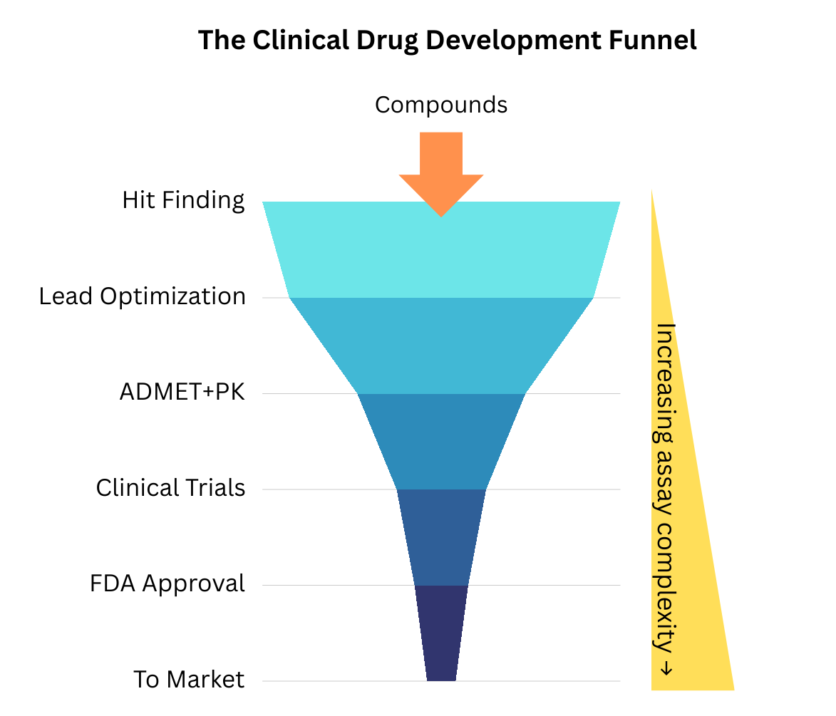
Traditionally, early-stage liver metabolism testing was performed in whole-organism systems (e.g., mice, rats, dogs) or with isolated liver cells (hepatocytes). Although more comprehensive, these approaches are expensive and difficult to standardize. Assay technology has since evolved, and testing can now be performed at high throughput using liver microsomes. While hepatocytes are intact, living cells that contain the full complement of metabolic enzymes, transporters, and cofactors to reflect "whole-cell" clearance, liver microsomes are subcellular fractions. They conveniently contain many of the membrane-bound enzymes responsible for drug metabolism: cytochrome P450s (CYPs), flavin monooxygenases (FMOs), and UDP-glucuronosyltransferases (UGTs). Microsomes are far easier to prepare and store than hepatocytes and are compatible with high-throughput methodologies and automated liquid handling. This makes them a simpler tool for assessing Phase I oxidative metabolism and has allowed liver metabolism testing to move down the cost curve and up the assay cascade (Figure 1), making it an endpoint routinely collected during lead optimization.

Beyond simple filtering within a lead series, these assays enable direct quantification of in vitro metabolic rates and, consequently, prediction of preclinical and First-in-Human (FIH) doses through In Vitro-In Vivo Extrapolation (IVIVE). This is the cornerstone of de-risking a lead, enabling medicinal chemists to identify metabolic "sweet spots,” estimate a first dosing schedule, and gauge expected metabolic behavior in subsequent PK studies.

Why Use a Predictive Model?

While microsomal assays are amenable to high-throughput automation, the sheer volume of chemical space explored during early discovery often outpaces laboratory capacity and financial resources. 

In silico modeling offers a high-efficiency alternative to physical screening by providing prioritization and enrichment. Early quantitative estimates of metabolic stability enable researchers to prioritize compounds with favorable PK profiles, ensuring that limited in vitro resources are focused on the most viable candidate molecules. This can save considerable time and effort downstream, where metabolic liabilities may have to be engineered out of much more developed molecules with complex synthetic routes.

At OpenADMET, we believe that democratizing these predictive tools is essential to streamlining drug discovery programs. To that end, we have developed an open-source microsomal clearance model based on public data designed to provide accessible ADMET predictions for the broader scientific community. Like our other models published to date, this model is a baseline. It represents a reasonable-effort attempt with publicly available datasets, not a model you should deploy in production with high confidence. Like other ADMET properties we are interested in, we would like to collect microsomal metabolism data at scale. Get in touch if this interests you! 

The Data

Before we dive into the actual modeling, it is essential to understand the data the model is learning from. Liver microsomal metabolism is quantitatively defined by intrinsic clearance (CL_int), which represents the liver's functional capacity to irreversibly remove a compound from circulation in the absence of physiological limitations. This parameter is typically derived from in vitro depletion assays, where the disappearance of the parent compound is monitored over a discrete time course. Under first-order linear kinetics—specifically when the substrate concentration [S] is significantly below the Michaelis constant (K_m)—the relationship simplifies to the ratio of the maximum reaction velocity to the affinity constant (V_max/K_m).

To translate these benchtop values into clinically relevant predictions, CL_int is integrated into physiological frameworks such as the Well-Stirred Model. This model treats the liver as a single, well-mixed compartment where the concentration of the drug leaving the organ is in equilibrium with the concentration inside. By incorporating biological variables—primarily hepatic blood flow (Q_H) and the unbound fraction of compound (f_u)—the model transforms raw enzymatic rates into a total hepatic clearance (CL_H).

Liver metabolism data in particular, can be tricky and has some nuances, such as units and scaling, that are not immediately apparent if you don’t have a background in PK or drug development. In particular, the units of CL_int can vary depending on whether you are referring to in vitro data, in vivo data or in vitro data that has been scaled with in vitro to in vivo extrapolation (IVIVE). The difference between these units of CL_int is obvious empirically. In vitro experiments are conducted in a controlled environment outside of a living organism, e.g. in a test tube, petri dish, or deep well plate. In vivo experiments are performed within a whole living biological system, e.g. a plant, animal, or human. With IVIVE, you can then transform between the two data scales.

If you pull microsomal clearance data from ChEMBL, you’ll notice units of ml/min/g, µl/min/mg, and ml/min/kg. This is where you have to proceed with caution: there are a couple of types of CL_int.

1. Microsomal or in vitro CL_int is usually the value directly output and measured by the assay. This typically has units of µl/min/mg or ml/min/g, which are equivalent. However, this number is not directly comparable to in vivo clearance data as it depends on the enzyme content present in the microsome.
2. In vivo CL_int, which has units of ml/min/kg and is derived either directly from in vivo experiments or by scaling in vitro microsomal data based on the average weight of the liver and the average weight of the whole body for the species’ microsome you’re using. This allows direct comparison to in-vivo PK for the relevant species data and is the input for the well-stirred model above. When pulling data from ChEMBL, it’s not often clear whether you are extracting correctly scaled in vivo CL_int values.

Warning! Although it looks like you can convert in vitro CL_int to in vivo CL_int by simply dividing by 1000, this is not the case. As mentioned, the scaling is based on the organism’s body and liver weight, and the appropriate scaling factors must be applied. The equation is:

Fortunately, the scaling factors, microsomal protein content and liver weight, are static reference values, and so conversion is fairly simple. As an example, to convert an in vitro CL_int of 300 ml/min/g from a human liver microsome (HLM) assay to in vivo CL_int, you would apply the relevant microsomal protein content (45 mg), average liver weight per kg of body weight (26 g/kg) and an estimate of the fraction unbound in microsomes (assumed to be 1 if not explicitly measured in a separate assay).

While this is a simple calculation, it can cause considerable confusion if you do not carefully check your units. Take this example (Figure 2) comparing unscaled and scaled data from ChEMBL and the Polaris-ASAP dataset, respectively. The data from ChEMBL is collated from a variety of sources, while the ASAP dataset is a focused single-source dataset from a lead optimization campaign. The unscaled ASAP data looks noticeably different from the ChEMBL data. Recklessly proceeding to model training at this point would result in inaccurate predictions and likely poor model performance. When we scale the ASAP data to in vivo CL_int using the equation described above, the ASAP data aligns more closely with the ChEMBL data (Figure 2B).

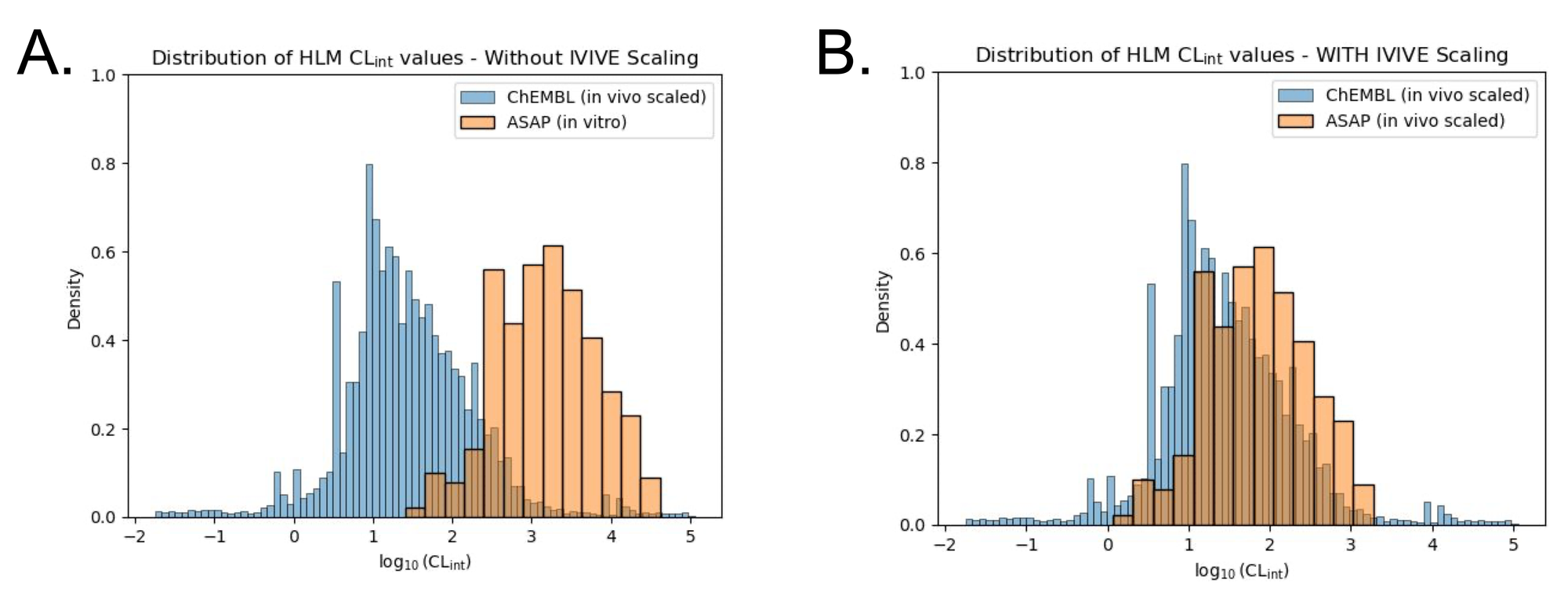
You’ll notice in these plots that CL_int has been log₁₀ transformed. This is because like most biological data, CL_int is heavily right-skewed and spans multiple orders of magnitude. Log₁₀ transformation reduces that skew and facilitates interpretation and modeling. Machine learning relies on certain assumptions of the underlying distribution of the data you’re training on, mainly that the data is roughly balanced and symmetrical. Training a model on heavily skewed data could lead to poor performance and biased predictions, hence a log-transformed model is often preferred. When performing inference, predicted log₁₀CL_int can be back-transformed to CL_int by taking the exponent. 

You may now be wondering why we bother with scaling to in vivo CL_int at all. Why can’t we just train a model to predict in vitro or microsomal CL_int? And we could, but frankly, in vivo CL_int is the scale that most clinical drug discovery professionals care about because it is immediately interpretable. For example, a seasoned expert will be able to immediately gauge whether a compound has low, moderate, or high clearance, relative to human liver blood flow rate. CL_int above liver blood flow rate often indicates the compound has high extraction and hepatic clearance becomes flow limited. When total systemic clearance exceeds blood liver flow, this generally suggests some kind of extrahepatic clearance, or metabolism outside of the liver. We believe these are all important considerations that can make the difference in promoting a hit compound to the next stage of optimization, but invite the community to share their expertise and opinions on this.

For our modeling experiments, we used our openadmet-toolkit package to query CL_int data from ChEMBL’s database for three species of most commonly used microsomes: human, rat, and mouse. We accounted for the different scales of CL_int reported by IVIVE scaling all values to in vivo. We then log-transformed the CL_int values and canonicalized the SMILES strings for every compound using our openadmet-toolkit package. The resulting datasets are available in our data catalog. 

Modeling Results

To find the best baseline model, we set up a matrix with several computational parameters to enumerate. Experiments were performed with our ANVIL training harness, allowing easy reproducible training across several model architectures.

1. Model architecture - We focused on three model architectures: the tree-based traditional machine learning model, LightGBM (with concatenated fingerprint + descriptor features), the transformer-based tabular model, TabPFN (same feature set as LightGBM), and the Chemprop-based GNN foundational model, CheMeleon, which can perform both single and multi-task predictions. These three model types have been our best-performing models for other ADMET endpoints and were performant in the recent OpenADMET challenge with ExpansionRx Therapeutics.
2. Splitting method for the data - We tried splitting our data for training (0.7), validation (0.1), and test (0.2) sets two ways: with a standard random split and a cluster split. The cluster split groups molecules that are chemically similar, so the model will be trained on one group and tested on a chemically different group. We were interested in seeing how well a model could generalize to unseen pockets of chemical space. Random splitting (easier) and cluster splitting (more difficult) represent reasonable guesses at upper and lower performance bounds for real-world predictions.
3. Benchmarking our model results on real datasets - We have a couple of high quality datasets from real drug discovery programs to benchmark our results against: the Polaris-ASAP, Biogen, and ExpansionRx Therapeutics datasets. These datasets were processed in the same way as our ChEMBL dataset: CL_int values were IVIVE-scaled if needed, CLint values were log-transformed, and SMILES were canonicalized the same way. We can then perform inference and compare our values to those measured in these campaigns.

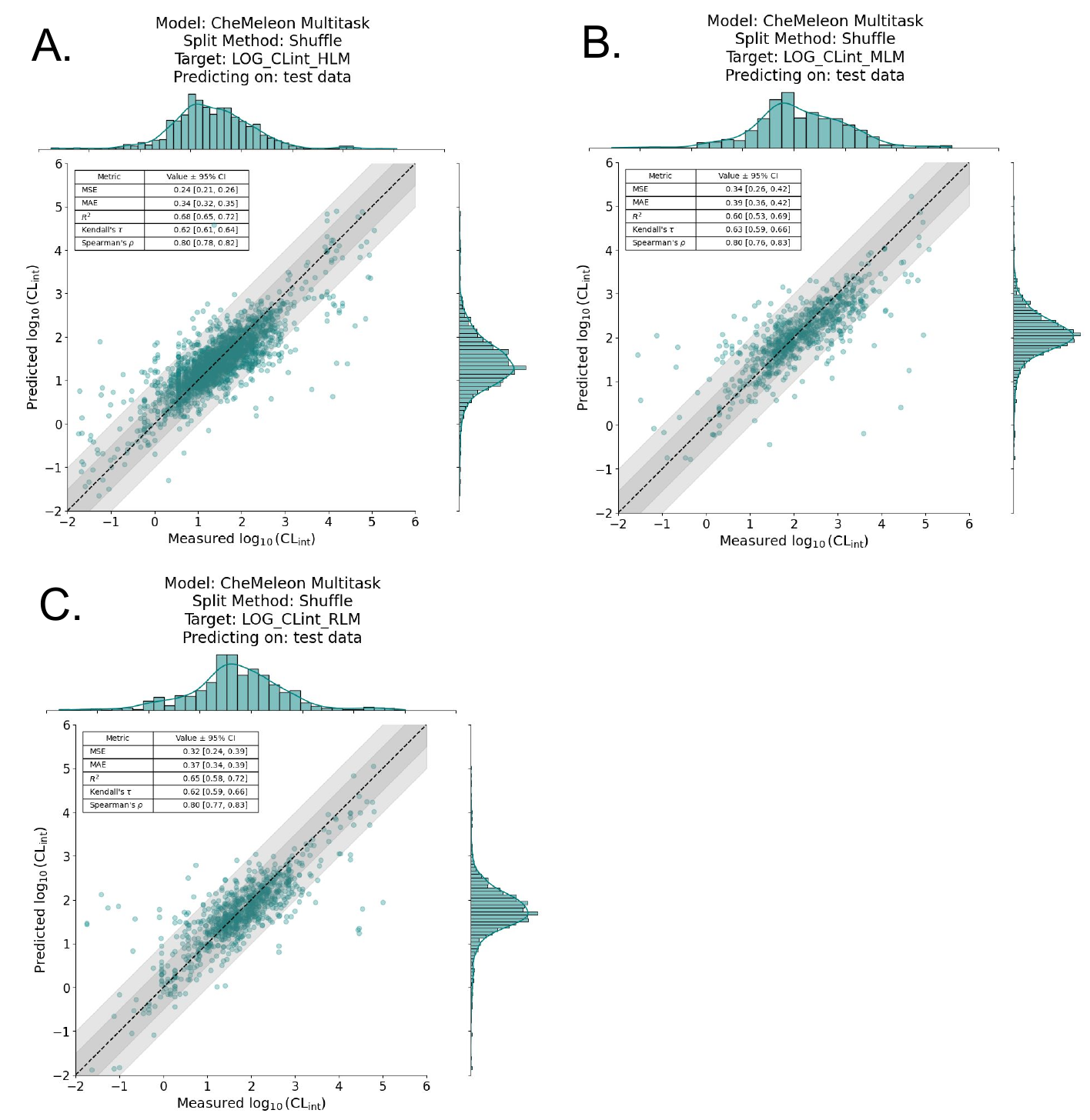
For each species of microsomal data (human liver microsome, rat liver microsome, and mouse liver microsome), we trained a model with each splitting method and with 5x5 cross validation. We found that the CheMeleon models with a random split performed better overall than those with a cluster split. Figure 3 shows the predictive results on the test set for each species; model performance is reasonable.

Important to note: the differences in performance between random and cluster split here can be misleading. Keep in mind our context is ADMET modeling. A random split usually assumes that the data points are independently and identically distributed, but this is clearly not the case here: molecules can be more or less chemically similar to one another. If very similar chemotypes appear in both the training and test datasets (as can happen with random splitting), the model’s task is interpolation, i.e., predicting within the same chemical space it was trained on.

On the other hand, cluster splitting splits the data based on structural similarity: molecules in the training set will be more dissimilar to the molecules in the test set. The model now has the much more difficult task of extrapolation, where it has to predict novel chemotypes. These two splitting methods represent the two ends of the spectrum for ADMET prediction: either predicting within a known part of chemical space, as you might when optimizing for a lead series, or predicting on an unknown or unseen part of chemical space, perhaps when you are still in the discovery phase and are looking for novel compound series for a new disease target.

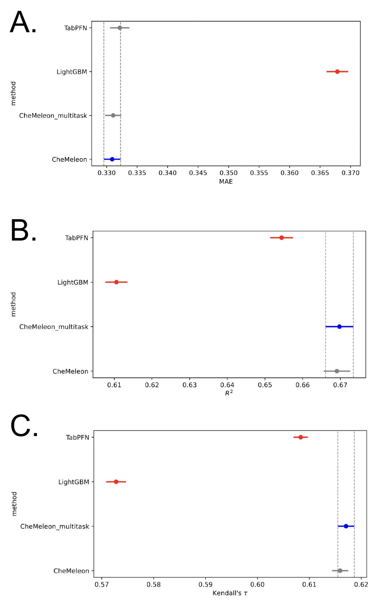
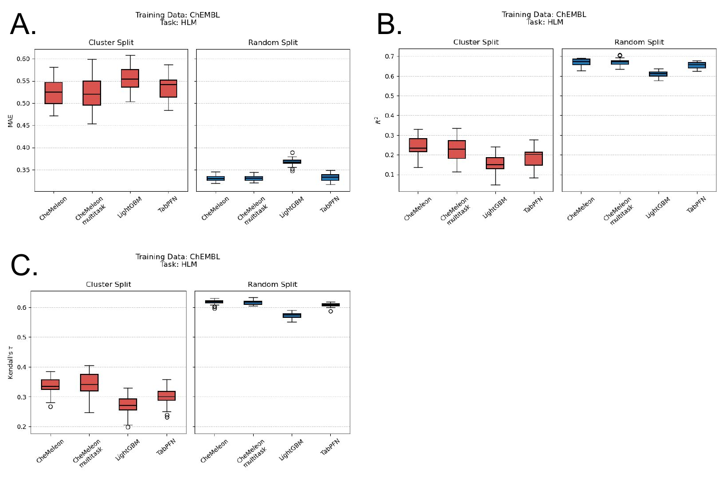
To rank among model performance, we compared all human liver microsome models using random splits in an ANOVA (Figure 4), following the statistical analysis procedure outlined here [6]. These plots show the statistical significance between a few key performance metrics: the mean absolute error (MAE), Kendall’s 𝛕, and R² value. The points in blue are ranked best for that performance metric, the gray points are not statistically significantly different from the top model, and the red points are statistically inferior to the top model (blue).

In totality, the CheMeleon model was superior to TabPFN and LGBMs, consistent with recent data from the ExpansionRx challenge (and our experience with other models). Multitask CheMeleon was not statistically superior to single-task CheMeleon, however it does offer an advantage in terms of convenience.

In contrast, we found that all of the models trained with a cluster split consistently performed worse than the random split method across all species and datasets (Figure 5). In other words, when the data was clustered by similarity, and the model was tested on a set of molecules that were dissimilar to the training set, the model's performance deteriorated significantly. This showed (once again) the difficulty of extrapolating outside the training set, a phenomenon well established in the literature. In quantitative structural activity relationship (QSAR) modeling, for example, people will use some method, usually a structural similarity function, in an attempt to ascertain how reliable a model’s predictions are. However, these methods are mostly rooted in intuition and ease of interpretability rather than scientific rigor or validity, and it remains one of the prevalent problems in the field of ADMET modeling.

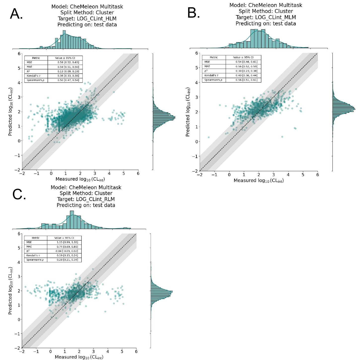
The poor performance of cluster-split models is even more evident in the regression plots (Figure 6). If we examine the model analogous to the best-performing model, multitask CheMeleon, but trained with a cluster split, the difference is stark.

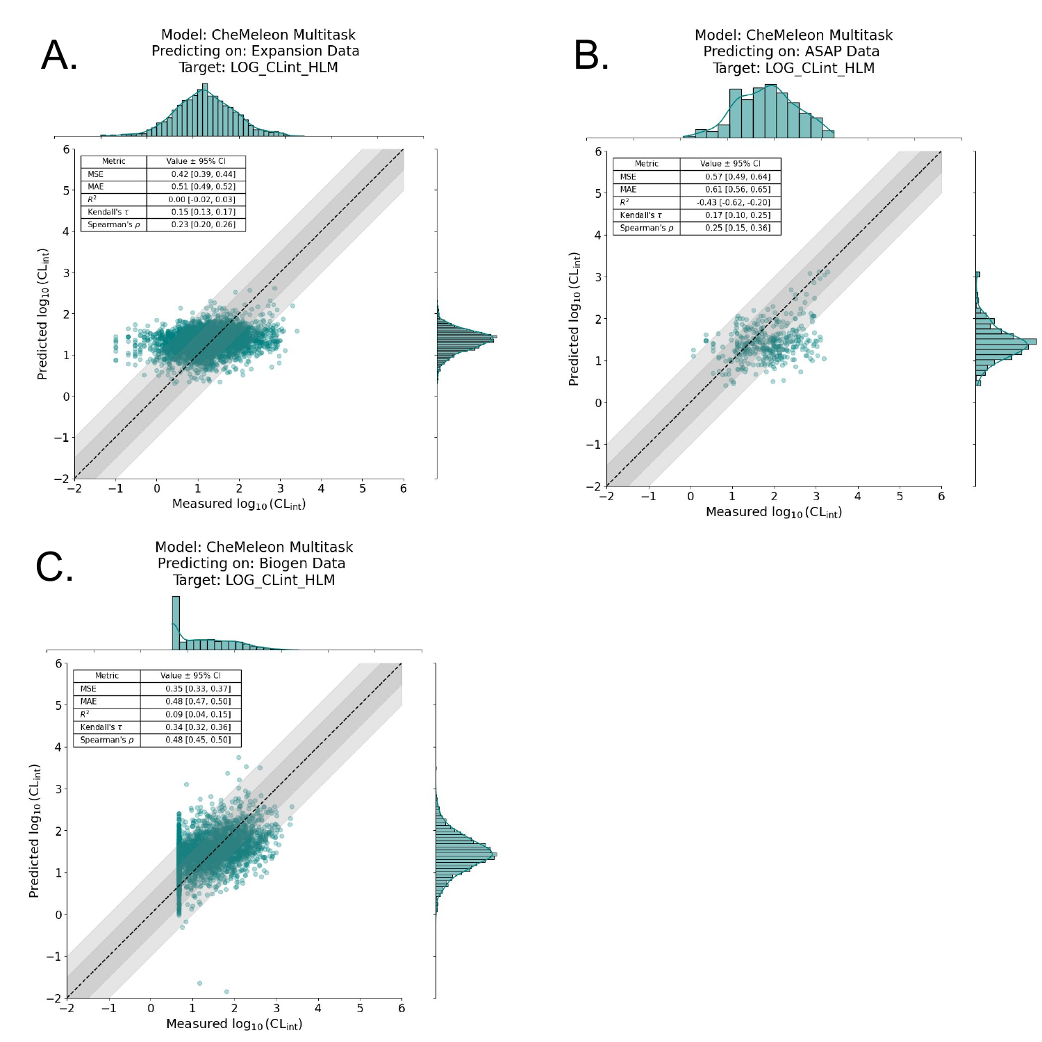
Given the multitask CheMeleon model’s superior performance, we trained a full production model, i.e. train=1.0 of all the ChEMBL data. We then assessed performance by predicting on the aforementioned benchmark datasets from Polaris-ASAP, Biogen, and ExpansionRx. Unfortunately but not unexpectedly, performance was quite poor. Figure 7 shows the regression plots for each benchmark, where the y-axis is our model’s predicted log₁₀CL_int value and the x-axis is the actual log₁₀CL_int value. While it appears our model detected a signal on the Biogen dataset (Figure 7C), it performs poorly on both the Polaris-ASAP and ExpansionRx datasets, which are much more focused chemical spaces around specific lead-like series (Figure 7A, 7B).

Why might this be? In our past modeling experiments with other endpoints, we observed a persistent trend: our models did not generalize well to regions of unseen chemical space. In other words, if a model is shown molecules to predict on, but there are no chemically similar molecules in its training data, the model performs poorly. This is a well-known phenomenon in the ADMET/QSAR modeling space, where models are ideally only used for interpolation within their applicability domain and not extrapolation.

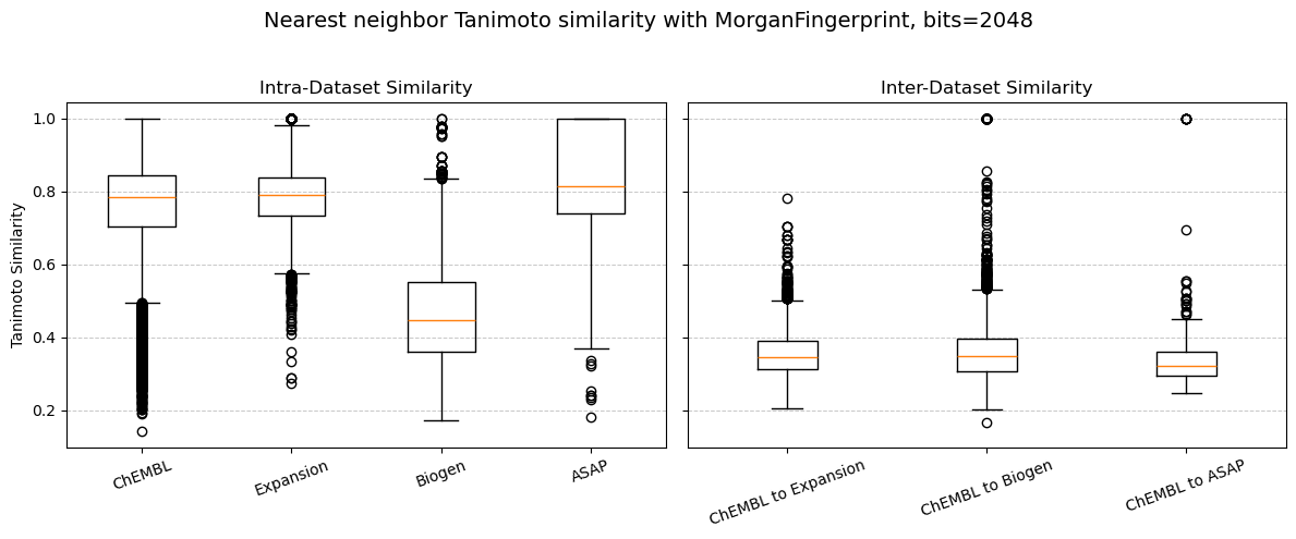
This is supported by a couple of observations in our experiment: When examining the nearest neighbour chemical (Tanimoto) similarity within each dataset, we find that the molecules within the ChEMBL, Expansion, and ASAP datasets are all very similar to each other with Tanimoto similarities closer to 1 (Figure 8, “Intra-Dataset Similarity”). This makes sense, given that the ExpansionRx and ASAP-Polaris are focused lead-like series and so will have mostly similar molecules. The Biogen dataset, in contrast, is a collection of 120 different datasets generated by Biogen over two years for multiple endpoints, and so is more chemically diverse (Tanimoto similarity ≈ 0.4).

However, when we compare across datasets, e.g. “ChEMBL to Expansion”, “ChEMBL to Biogen”, and “ChEMBL to ASAP”, we find that all our benchmark datasets are very dissimilar to the ChEMBL dataset with Tanimoto similarities of < 0.4 (Figure 8, “Inter-Dataset Similarity”), meaning that the part of chemical space that our model was trained on (ChEMBL) is not at all similar to the datasets we’re predicting on (Expansion, Biogen, and ASAP). This is a possible explanation for how poorly the CheMeleon multitask model performs on benchmark sets: the model is only reliably and/or accurately predictive on the chemical space it was trained on.

This concept is known as applicability domain and is a prevalent and ever-evolving topic within the ADMET modeling field. We won’t dive into it too deeply here, but keep an eye out for a future blog post that does.

Conclusion

We are excited to expand our modeling capabilities to new PK endpoints, given the non-trivial challenges associated with ADMET modeling, e.g., curating the data alone is difficult and, as shown here, requires specific domain knowledge to accurately capture data nuances.

Again, the model shown here is a baseline, not a production-grade model with high accuracy across wide swaths of chemical space. We’ve done our best with the publicly available data, and these initial results look promising, but there is much further work to be done to improve microsomal clearance modeling.

Our experiments have once again reinforced that models perform well only within the pockets of chemical space they were trained on, and that generalizability is often poor outside those pockets unless we can add additional data for fine-tuning. Looking forward to future blog posts about the applicability domain in further detail!

Where’s the model?

Our baseline model is available for you to try out! Check it out here.