Are tabular foundation models all you need?
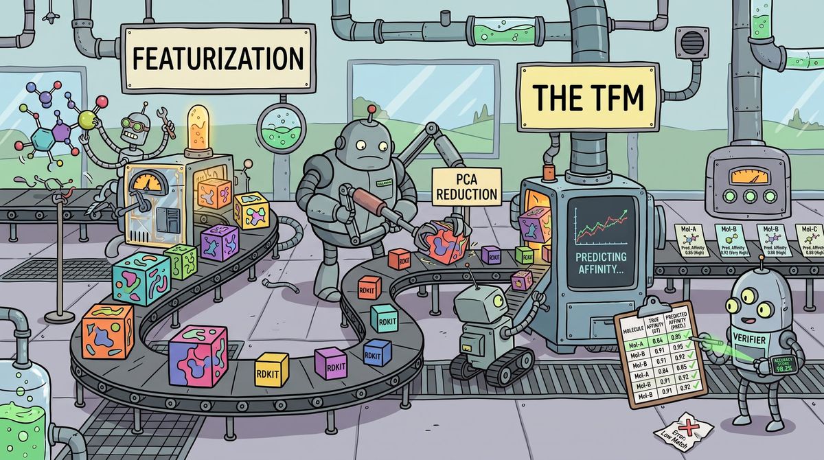
After the PXR blind challenge, we found that feeding a CheMeleon embedding and primary screen predictions into a tabular foundation model drove a top entry's accuracy. The combination cut our MAE from 0.50 to 0.43 and is now a first-class pipeline in openadmet-models.
Authors: Sean Colby
DOI: pending
The OpenADMET PXR (pregnane X receptor) blind challenge has closed, and the top of the leaderboard was ripe with highly performant submissions. At challenge end, a paired-bootstrap analysis could not separate the top entries. Our own model catalog was not among them, so we did what any curious team does after a challenge: we read the top participants' reports, looking for ideas to implement.
We ran the PXR blind challenge from April through July 2026, ending with thousands of submissions from more than 350 unique participants, 28 of which were statistically indistinguishable at the top of the leaderboard. Our CheMeleon baselines, implemented in openadmet-models, were starting to look a bit long in the tooth by comparison, landing around 0.50 MAE (mean absolute error), well below the ~0.41 MAE achieved by the leading entries. Consequently, we decided to explore alternatives.
In our search, we did not prioritize the lowest score alone. Large ensembles tuned over many submissions might nab the top leaderboard slot, but we wanted something we could fold into openadmet-models as a reproducible pipeline defined in YAML (yet another markup language): a method disclosed in enough detail to rebuild, and simple enough to maintain after the dust settled. Numerous unique ensemble members, each with its own weights and featurization to package, version, and rerun, are a lot to maintain.
The entry from participant N283T (model report) did both: a full-fledged nine-member ensemble (five frozen graph encoders, two Boltz-2 structural models, and two tabular models) with a Caruana-weighted forward selection and a fairly performant non-ensemble solution. Their leaderboard entry achieved an MAE of 0.41 on the blinded 260-compound Phase 2 set, crediting the core idea to Buterez et al. 2024 (Nature Communications), a multi-fidelity transfer-learning paper. The premise is appealing: cheap, abundant low-fidelity labels can serve as a proxy to sharpen predictions for the scarce, expensive high-fidelity target we actually care about. It also maps cleanly onto the PXR assay funnel, where thousands of single-concentration log2 fold change (log2FC) primary-screen readings sit upstream of a few thousand dose-response half-maximal effective concentration (EC50) values. We assumed the Buterez paper's architecture was driving the performance, and set out to reproduce it.
Upon reading the report closely and rebuilding the pieces ourselves, however, we found that the Buterez paper contributed a single, albeit important, component: an auxiliary encoder trained on primary-screen data to predict a log2FC readout. The paper's architectural configurations, the frozen and fine-tuned graph-network configurations we compared in Figure 1, did not produce the sought-after improvement. Instead, the gain came from feeding the log2FC readout columns, alongside a molecular embedding, into a tabular foundation model (TFM). N283T reached the same conclusion in their own analysis, finding the log2FC-trained Chemprop embedding to be their single strongest feature when used as input to a TFM.
That combination, careful featurization feeding a TFM, reduced our MAE from ~0.50 to ~0.43 on this split, a step large enough that we wanted to support it as a first-class configuration in openadmet-models. In this post, we work through what each ingredient contributes in isolation, how the ingredients combine into the best performer, and which TFM performs best.
Graph-network baselines
We evaluated several approaches that use a graph neural network (GNN) rather than a tabular foundation model, following the transfer-learning strategies from Buterez et al. 2024:
- Chemprop, and the CheMeleon foundation initialization, trained against pEC50 (baselines)
- A log2FC-trained embedding network, which we do not score directly but which feeds the two configurations below (Buterez's E1)
- An auxiliary-encoder-plus-concatenation design, wherein the outputs of a log2FC-trained Chemprop are concatenated into the primary network before the feed-forward network (FFN) (Buterez's E3)
- Chemprop / CheMeleon initialized from the log2FC-pretraining checkpoint, then trained against pEC50 (Buterez's E4)
- We omitted Buterez's E2, which concatenates the measured log2FC labels rather than a model's estimate of them
The best of these was Chemprop initialized from the log2FC checkpoint and fine-tuned to pEC50 values, nominally ahead of the single-stage CheMeleon baseline and the best concatenation configuration. Nothing on the panel is separated from the best row: the Tukey Honestly Significant Difference (HSD) critical distance across the ten configurations is 0.10 MAE, and the closest comparison is p = 0.62. None of these experiments reached the accuracy N283T reported.
Figure 1. Graph neural network implementation performance. Test set MAE in ascending order for the graph-encoder configurations evaluated in this work; each point is the mean across 5 random seeds. Whiskers are Tukey HSD comparison intervals, blocked on seed. Overlapping whiskers signal that a pair cannot be distinguished. The shaded band spans the best row's interval. The N283T row is a published leaderboard value, drawn without an interval and not tested against. Hover over a point or row label to see detailed configuration information.
What are tabular foundation models?
A bit discouraged by the GNN results, we turned to the next potential source of improvement: using a TFM as a regressor. But what are they, other than "a foundation model for tabular data"? Prior to this effort, Karim Ben Hicham gave an excellent overview in our OpenADMET seminar series, based on his work detailed in this paper. In summary, TFMs are pretrained on millions of synthetic tables whose data-generating process is known by construction, learning to approximate Bayesian inference. Performing exact Bayesian inference is computationally intractable because it requires integrating over the entire space of possible data-generating models. Consequently, estimating this inference in a single forward pass, keeping training instances directly in context without fitting model parameters, offers an elegant way to reduce compute time and resources... But does that pretraining generalize to the relationships under study here?
Reducing dimensionality
The next sections turn to TFM evaluation, which is notoriously memory-intensive. Descriptor sets reach 217 dimensions for RDKit, 1,613 for Mordred, and a CheMeleon embedding 2,048, with combinations even larger. To avoid overflowing memory, we turned to Principal Component Analysis (PCA). PCA is a technique that reduces the number of variables in a large dataset while preserving variance. We swept PCA dimensionality reductions across descriptors and fed them to TabPFN in isolation to test whether we could safely reduce the feature count without degrading performance (Figure 2, left). Native-dimension RDKit led the comparison at 0.53 MAE, but was statistically indistinguishable from PCA-reducing it to 128. Mordred and RDKit+Mordred trailed in all tested configurations. We therefore proceeded with RDKit descriptors PCA-reduced to 128 dimensions as our canonical descriptor set.
We performed a similar sweep with the 2,048-dimensional CheMeleon embedding (Figure 2, right). We could not evaluate dimensions above 512 because of memory limits. PCA reductions to 256, 384, and 512 were statistically indistinguishable, while 128 and below were clearly separated and performed worse, so we chose 256 dimensions as our canonical PCA-reduced CheMeleon embedding.
Figure 2. Dimensionality reduction impact. Left, descriptors: test set MAE varying the descriptor set (RDKit, Mordred, or both) and its PCA width (32, 64, 128, 256 components, or native). Right, embedding: the CheMeleon embedding at 32 to 512 components. Overlapping whiskers signal that a pair cannot be distinguished. The shaded band spans the best row's interval. The N283T row is a published leaderboard value, drawn without an interval and not tested against. Hover over a point or row label to see detailed configuration information.
Individual ingredient contributions
We then tested each candidate ingredient individually using TabPFN v3 as the regressor, as shown in Figure 3. The embedding from a CheMeleon encoder fine-tuned on log2FC was the nominally best single-ingredient result here, tied with the off-the-shelf CheMeleon embedding, the pEC50-trained CheMeleon embedding, the log2FC-trained Chemprop embedding, and the best graph network configuration from Figure 1. Remaining configurations, including the single-stage CheMeleon baseline, are all significantly worse.
Figure 3. Single-ingredient into tabular foundation model performance. Test set mean absolute error (MAE) for each candidate feature in isolation, fed to TabPFN v3. Overlapping whiskers signal that a pair cannot be distinguished. The shaded band spans the best row's interval. The N283T row is a published leaderboard value, drawn without an interval and not tested against. Hover over a point or row label to see detailed configuration information.
Combining embedding, log2FC readout, and descriptors
We evaluated every subset of embeddings, log2FC readouts, and descriptor sets across five embeddings (CheMeleon off-the-shelf, CheMeleon fine-tuned on log2FC, CheMeleon fine-tuned on pEC50, and Chemprop trained from scratch on either target) and the two log2FC readouts provided by those encoders. Looking at Figure 4, the nominal best configuration was the log2FC-fine-tuned CheMeleon embedding + Chemprop log2FC readout + RDKit 128 descriptors, statistically tied with fifteen of the thirty-six rows. Three such configurations omit descriptors entirely, suggesting the descriptor block adds no detectable value beyond an embedding plus log2FC readout. The best single-ingredient configuration, the log2FC-trained CheMeleon embedding, is also statistically tied, which calls readout inclusion into question. The remaining embedding-only configurations are statistically worse, as are the best graph network and the CheMeleon baseline. We carried forward the off-the-shelf CheMeleon embedding + Chemprop log2FC readout, which ties the leader while keeping the implementation much simpler, though the case for retaining the readout was weak.
Figure 4. Feature combinations into tabular foundation model performance. Test set MAE for every subset of the three ingredients (embedding, log2FC readout, and descriptors), all fed to TabPFN v3. Overlapping whiskers signal that a pair cannot be distinguished. The shaded band spans the best row's interval. The N283T row is a published leaderboard value, drawn without an interval and not tested against. Hover over a point or row label to see detailed configuration information.
Evaluating tabular foundation models
With the feature set fixed to off-the-shelf CheMeleon embedding + log2FC readout, we swapped only the regressor to test whether a different tabular foundation model (or gradient boosting model) could beat TabPFN v3 on the same inputs. TabICL comes out nominally ahead, tied with TabPFN v3. TabFM, LightGBM, XGBoost, and TabPFN v2.6 are all separated from the leader.
We note that TabFM's number is not fully comparable: max_num_rows is capped at 500 in TabFM v1.0.0 because the full 4,392-row training set hits memory limits during its attention pass on the graphics processing unit (GPU) used here, so its in-context set is subsampled per ensemble member, whereas TabPFN and TabICL could accept all 4,392 rows.
As noted above, TabICL only narrowly leads TabPFN v3, with a seed mean of 0.427 versus 0.436. However, TabICL is licensed under BSD 3-Clause, while TabPFN uses the Prior Labs Licence, Apache 2.0 with an added requirement to display "Built with PriorLabs-TabPFN" on any related website, blog post, or product documentation, as well as a TabPFN name prefix on models derived from it (as applies to this very post). As the "Open" in OpenADMET suggests, we prefer the more permissive license when all else is equal. TabICL does have its own drawbacks, though: it did not fit within our 24 GB GPU memory budget and fell back to the central processing unit (CPU), taking about 184 seconds per run, compared with 14.6 seconds for TabPFN v3 on the GPU for the same task. TabICL at 128 dimensions does fit on the GPU, at about 13 seconds per run.
Figure 5. Tabular foundation model comparison. Test set MAE with the feature set held fixed (CheMeleon embedding + log2FC readout), varying only the tabular foundation regressor. The swept rows cover two TabPFN releases (v2.6 and v3), TabICL, TabFM, and two gradient-boosted baselines (LightGBM and XGBoost). Overlapping whiskers signal that a pair cannot be distinguished. The shaded band spans the best row's interval. The N283T row is a published leaderboard value, drawn without an interval and not tested against. Hover over a point or row label to see detailed configuration information.
Do tabular foundation models quantify uncertainty well?
Tabular foundation models also produce a predicted distribution for each compound. TabICL reports this as quantiles, and we converted the 10th-to-90th percentile span into a normal-equivalent standard deviation. We used the off-the-shelf CheMeleon embedding + log2FC readout fed into TabICL to assess whether these predicted distributions help with uncertainty quantification, the subject of a previous OpenADMET post. Figure 6 (left) plots each compound's absolute residual against its predicted standard deviation, testing whether predicted standard deviation correlates with error. Figure 6 (right) plots empirical coverage against nominal level across 99 quantile levels to test whether, for example, the predicted 0.4 quantile actually has 40% of true values at or below it. Perfectly calibrated predictions would track the diagonal; an overconfident model below it, an underconfident model above it.
The spread did track error, but only weakly: the Spearman rank correlation (ρ) between predicted standard deviation and absolute residual was 0.26. Recalibrating the quantiles would not raise that correlation, because Spearman ρ is rank-based and invariant to any strictly monotonic rescaling of the predicted standard deviation. The intervals themselves are close to the right width, with a miscalibration area of just 0.04. Thus, in this case, tabular foundation models give us well-calibrated intervals of roughly the right width, but not a reliable ranking of which compounds are uncertain / hard.
Figure 6. Predicted uncertainty versus actual error. Left: each of the test compounds' predicted standard deviation, plotted against its absolute error. Right: the reliability diagram, observed coverage against nominal coverage across 99 levels, with the dashed diagonal marking perfect calibration.
Applying the method to the CYP inhibition blind challenge
OpenADMET's next blind challenge, modeling cytochrome P450 (CYP) inhibition across 4 isoforms, kicked off on August 17, 2026. Of course, we wanted to apply the newly minted approach. Off-the-shelf CheMeleon embedding + log2FC readout is the TabICL-baseline, which held the top spot on the regression live leaderboard—ranked by mean-averaged, standardized target, relative absolute error (MA-ST-RAE)—for... a few days (0.68 MA-ST-RAE). As of this writing, the top performers have reduced that error by ~36% (0.43 MA-ST-RAE). Still, the new method improves upon previous openadmet-models baselines by ~20% in this challenge (see the leaderboard's CheMeleon-baseline at 0.83 MA-ST-RAE), well worth the effort to adopt.
Updating openadmet-models
To realize the PCA-transformed CheMeleon embeddings concatenated with log2FC predictions, as input into a tabular foundation model (exhale) in openadmet-models, we implemented several new features.
- A
CheMeleonFeaturizerto produce the off-the-shelf, 2,048-dim CheMeleon embeddings. - A PCA transformer that can be applied to all, or groups of, features listed in the featurization section of an anvil YAML. Or pass
Nonefor a given featurizer to enable direct passthrough of a subset. - A
PretrainedModelFeaturizerto read a trained model back in with another workflow to use that network's predictions as features. For example, train a Chemprop model on primary screen log2FC data, whose output then gets read into the main tabular foundation model as predicted log2FC features. - A
TabICLRegressor(andTabICLClassifier), to use TabICL for final predictions.
The pipeline can now be specified with just two YAML files, with example configs up on optimus-prime.
Reproducibility
All supporting code lives in the blog post repository. experiments/manifest.yaml is the spine: it declares every sweep, gate, and figure before anything runs, along with the axis levels this work deliberately excluded and why. src/manifest.py reads it, src/gates.py records the decisions, src/regressors.py and src/encoders.py build the models, and src/panels.py and src/plots.py produce every figure in this post. src/tukey.py computes the comparison intervals seen in the figures. The numbered scripts in run/ are the entry points, in the order they run.
To reproduce, install the dependencies with uv and run from the repository root:
uv sync

# Data, split, features, and reductions (all cached and content-addressed)
python run/00_fetch_data.py
python run/01_build_split.py
python run/02_featurize.py
python run/03_reduce.py

# Each stage sweeps, then aggregation writes the gate the next stage reads
for stage in descriptor_width embedding_width ingredients regressor tabpfn_ensemble; do
    python run/04_sweep.py --stage "$stage"
    python run/05_aggregate.py
done

# The graph networks depend on no gate and can run at any point
python run/04_sweep.py --stage gnn

# Uncertainty diagnostics on the chosen configuration, then every figure
python run/07_uncertainty.py
python run/08_figures.py
Acknowledgements
We would like to thank our funders for their support of OpenADMET, in particular ARPA-H, Radial (part of the Astera Institute), Schrödinger Inc, and the Gates Foundation. We would also like to thank our partners Enamine, HuggingFace, OpenEye, CDD Vault, Discovery Life Sciences, and the beamline staff at NSLS-II for their support.
This work is supported by the Advanced Research Projects Agency for Health (ARPA-H) under AVOID-OME, and Award Number 1AY1AX000035. The contents are those of the authors. They may not reflect the policies of the Department of Health and Human Services or the U.S. government. The content is solely the responsibility of the authors and does not necessarily represent the official views of the Advanced Research Projects Agency for Health.