Author: Cynthia Xu

DOI:https://doi.org/10.5281/zenodo.22132985

What is Applicability Domain (AD)?

Training machine learning (ML) models to predict ADME (Absorption, Distribution, Metabolism, Excretion) endpoints is a difficult but worthwhile effort that could potentially accelerate and streamline drug discovery. Unfortunately, this challenge comes with an added layer of complexity known as the applicability domain.

To explain with an example: let’s say you are working in a drug discovery program. At the start of the program, you’ve collected experimental data from a broad and diverse set of compounds. You want to use it to train an ML model to predict an endpoint, e.g., lipophilicity (LogD). As the drug discovery program continues, you find yourself narrowing in on a certain group of chemistries for one reason or another, e.g., they’re more potent, have more desirable properties, etc.

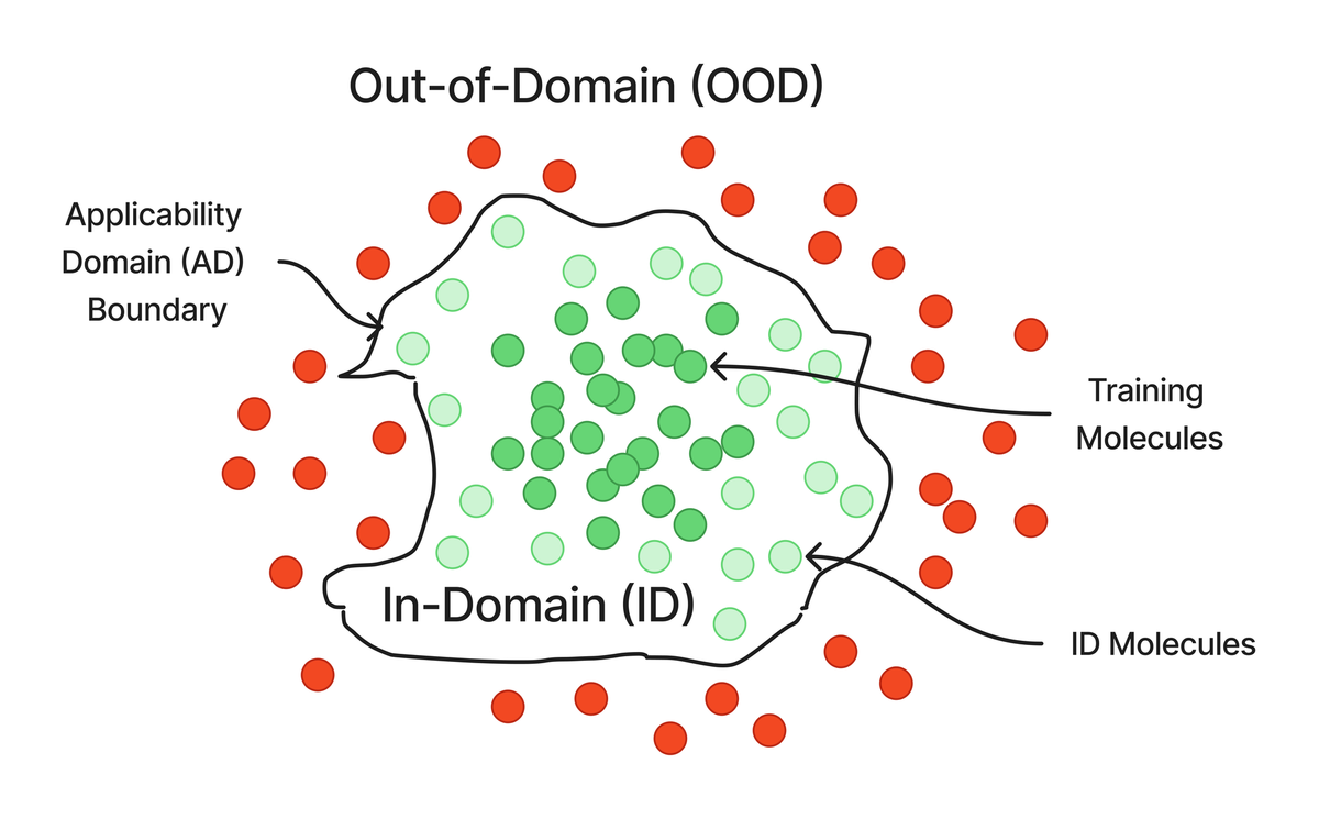
If you try to use the ML model you originally trained on the broader set of compounds, you may find that its predictions on the more specific set deviate considerably from the true experimental values. This is the concept of the applicability domain (AD) boundary; see Figure 1. Compounds in the model’s training set are in-domain or in-distribution (ID), meaning they fall within the model’s applicability domain, and the model can make reasonably accurate predictions for similar unseen molecules. Outside the AD boundary, however, molecules are out-of-domain (OOD), and the model will likely fail to provide reliable predictions for them. Critically, for unlabelled molecules where you do not have a ground truth assay result, a predicted value on its own does not tell you a priori whether a molecule is in or out of domain. This makes it difficult to trust model predictions, which is essential for practical use of models in a drug discovery campaign and a major source of experimentalist frustration. Now, your next logical question might be: how could I draw that boundary line? How do I define the AD of my model? Unfortunately, there is no simple or universal answer. The AD boundary is continuous and often very difficult to define. In this blog post, we explore some ways AD can be defined and how it may or may not correlate with model error.

Some ways to define AD

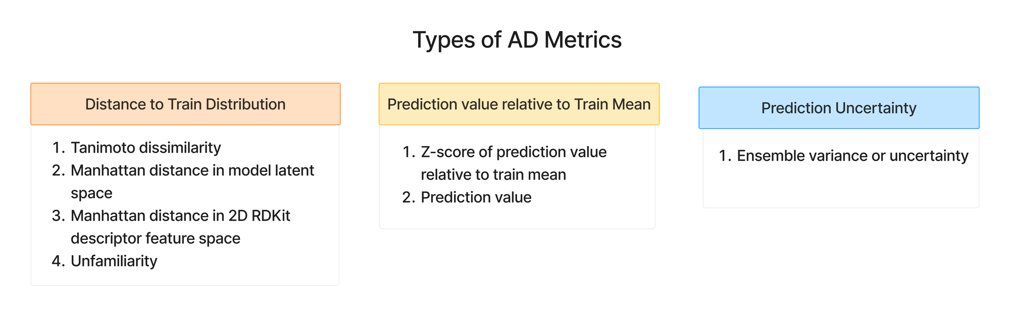
There are many ways to think about and define AD, but they generally fall into three main categories: distance from the training distribution in feature (or embedding) space, location in target variable or prediction space relative to the training distribution, and prediction uncertainty, as shown in Figure 2.

Distance from Training Distribution

Distance from the training distribution is probably the most intuitive concept for most people when thinking about AD. In essence, you are asking: how similar is the test set (what your model is predicting on) to the training set (what your model was trained on)? In computational drug discovery, this similarity is usually measured as a distance in a feature or embedding space between the training and test sets. It is reasonable to assume that compounds that are closer to your training set will be more ID for your model than compounds that are very distant. The four distance metrics we will consider in this work are shown in Figure 2 (leftmost column).

There are many ways to define this distance. One common example is chemical (Tanimoto) similarity between binary fingerprints, for example Morgan fingerprints. Test compounds classified as ID would be more chemically similar to the compounds in the training set. Our previous example shows this: the initial diverse compounds screened early in the drug discovery process and used to train the model are very chemically dissimilar to the later-optimized compounds you’d want to predict. Your model is therefore unlikely to give you reliable predictions on the later compounds. This is why it is important to keep updating your models dynamically as a campaign progresses.

While Tanimoto similarity is widely used, you can use any number of combinations of feature space and distance metrics. A few others we consider in this work are the Manhattan distance in both the 2D RDKit descriptor space and the model latent space, as done by Parrondo-Pizarro, R. et al. (2026) in their uncertainty quantification (UQ) work. 2D RDKit descriptors are just another molecular representation of compounds that capture physical properties, such as molecular weight and lipophilicity. Distance in the model latent space differs in that, rather than being fixed as they are for 2D descriptors, the representations are learned. The model architecture we’re using, ChemProp, has a forward pass that featurizes a compound’s SMILES string into a molecular graph. The directed message-passing neural network (D-MPNN) transforms that graph and aggregates it into a 300-dimensional learned embedding. The distances between these learned embeddings are what's computed as "distance in model latent space." The intuition for using this is that distances in the space the model was trained on may be more directly correlated with model performance than distances in a fixed, external feature space. However, in practice the two are already highly correlated, so you may not lose much by using either.

Another approach to calculating the distance to the training set is to use unfamiliarity, or reconstruction error. Proposed by van Tilborg, D. et al. (2025), this metric captures a different kind of distance learned by a model. An autoencoder is trained on the SMILES strings in the training set, compressing each SMILES string into a latent vector and then reconstructing it from that vector. When the autoencoder is asked to reconstruct SMILES strings from the test set, the accuracy of that reconstruction is the reconstruction error. For “familiar” molecules, or molecules very similar to the train set, the autoencoder should do a very good job of reconstructing them. Conversely, “unfamiliar” molecules will have a larger reconstruction error and are therefore more likely to be OOD. Unlike Tanimoto similarity, which relies on predefined fingerprint features, unfamiliarity quantifies distance using learned representations that may capture patterns not encoded in standard fingerprints. Unlike the model latent-space distances described previously, which are derived from the property prediction model itself, unfamiliarity is learned by a separate autoencoder trained solely to reconstruct SMILES strings, with no property prediction objective. However, because this is not the representation used to build the model, it can potentially suffer from the same issues as Tanimoto similarity.

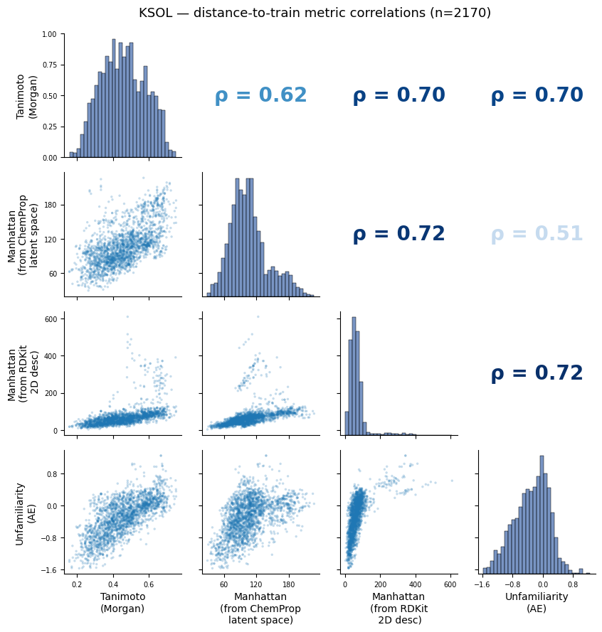
Figure 3 shows how these different metrics compare with one another. Although they all measure some form of “distance to the training set”, they do not strongly correlate with each other. They may broadly agree in most cases (ρ=~0.7), but they diverge at the extremes. This is especially important when defining AD because OOD compounds are likely to fall at the extremes of the distribution. How OOD compounds are classified will therefore depend heavily on the AD metric you use, and as you’ll soon see, there is rarely a one-size-fits-all AD definition.

Prediction value relative to Training Mean

Prediction value relative to the training distribution is another type of AD metric. This definition essentially asks where the predicted endpoint value for a test compound falls within the training distribution of endpoint values. Presumably, the farther the predicted test value is from the mean of the training distribution, the more OOD the test compound is. Some ways this can be operationalized are the absolute z-score, the number of standard deviations from the mean, or simply the prediction value itself. 

You might be wondering how to use the prediction value in this context. A quick spoiler: we examined several definitions of AD and found that the baseline metrics alone were not well correlated with model error, so we explored an alternative approach: training a separate model that uses multiple AD metrics, including the prediction from the ADME model, to predict error.

Prediction Uncertainty

Prediction uncertainty is a model-based AD metric and is also quite intuitive. Prediction uncertainty is how confident your model is about a given prediction, usually quantified as standard deviation or variance. A common way to calculate uncertainty is using model ensembles. In this work, we created an ensemble of n=5 models, with several replicate models initialized from different seeds. When predicting on the test set, all five models make predictions. Those five predictions are averaged to produce a point estimate, and the standard deviation of those predictions is reported as the uncertainty. When a model ensemble makes a prediction on a new test molecule, it produces a point estimate, but that single value should be more realistically interpreted as a range defined by the standard deviation. A large standard deviation on a prediction means the true value can fall anywhere within that range, and that the model is very uncertain about this prediction. High uncertainty may indicate OOD. Conversely, low uncertainty would, optimistically, mean that the compound is ID. 

An example with ExpansionRx data

Given all these options for defining AD, you may be wondering: how do I know which definition to use? Does one definition broadly apply to all endpoints? Or do I need to determine which AD definition is most appropriate for each endpoint I’m interested in?

We explored these questions using the ExpansionRx dataset, which was featured in one of our previous blind challenges. This dataset came from a real drug discovery program and collected common ADME endpoints for candidate compounds during lead optimization. For each of the nine endpoints with sufficient data, we trained a 5-member ChemProp ensemble to predict that property. This gave us both the predicted value for the endpoint and the model uncertainty (the predictions from each of the five members were averaged, and the standard deviation was calculated).

We then calculated the baseline AD metrics listed in Table 1 and examined the correlations between these metrics and the model’s absolute residuals (|y_pred - y_true|) across nine endpoints. To ensure statistical robustness, we performed 5x5 cross-validation on the test set to obtain a range of Spearman’s correlation coefficients for each endpoint. This lets us run a Tukey HSD test to determine whether one AD metric is significantly better than another. Other methods for generating a range of Spearman’s correlation coefficient values, such as bootstrap sampling, do not draw independent and identically distributed samples that would support a valid Tukey HSD test.

Table 1. Descriptions of the calculated baseline AD metrics and their typical ranges, including what is considered ID vs. OOD.

Figure 4 shows the Spearman’s correlation coefficients between each computed AD metric and the model’s error. We performed Tukey HSD comparisons for each metric at each endpoint to rank the best-correlated metric, as shown in blue. Points in gray are not statistically significantly different from the best, while points in red are. 

Overall, the correlations are low, and there is substantial variation across endpoints. With the exception of KSOL, the best-ranked AD metric has a correlation coefficient of less than 0.6. Unfamiliarity is the statistically best-ranked AD metric for 3 of 9 endpoints with no ties. This suggests that there are some advantages to learning distance from the training set with a model that are not captured by Morgan fingerprints, on which Tanimoto similarity relies. Uncertainty is the most compelling metric for KSOL, with ρ ≈ 0.6, but it is tied with either unfamiliarity or top-5 Tanimoto similarity for most other endpoints. MGMB has no clear winning AD metric, but this endpoint also has the fewest data points, so its correlations are noisier overall.

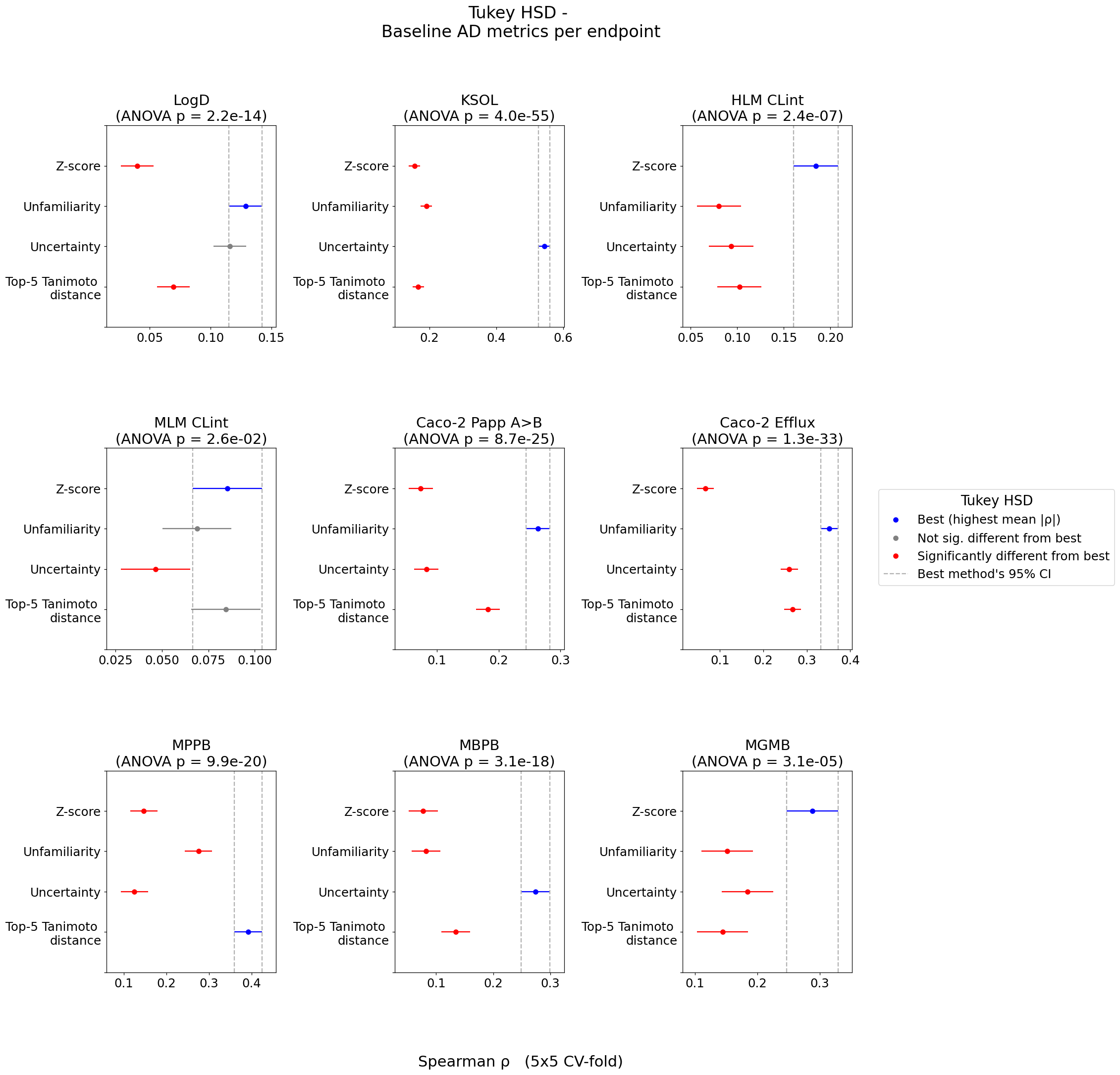
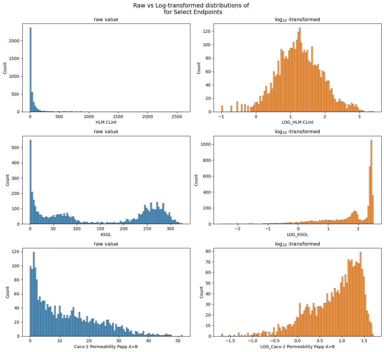
The z-score is consistently the statistical metric least correlated with AD across all endpoints. This is likely due to the nature of ADME data, which is often heavily skewed. The usefulness of z-score as a metric depends on the underlying distribution being approximately normal. All nine endpoints shown here had to be log-transformed before model training. In Figure 3, you can see several examples of endpoints before and after log transformation. Some endpoints, such as HLM CLint, become approximately normal after log transformation, but others, such as KSOL and Caco-2 Papp A>B, remain skewed even after log transformation. It is therefore unsurprising that we see the lowest correlation with the z-score. This AD metric just isn’t appropriate for this data context.

Learning AD with Error Models

We have shown that the raw baseline AD metrics alone do not strongly correlate with model error. A natural next question is whether combining AD metrics could instead train an entirely separate model to predict error, as in Figure 6. What isn’t possible with one may be possible with many. To do this, we drew heavily on the work of Parrando-Pizarro, R. et al (2026) and their UNIQUE library and pipeline.

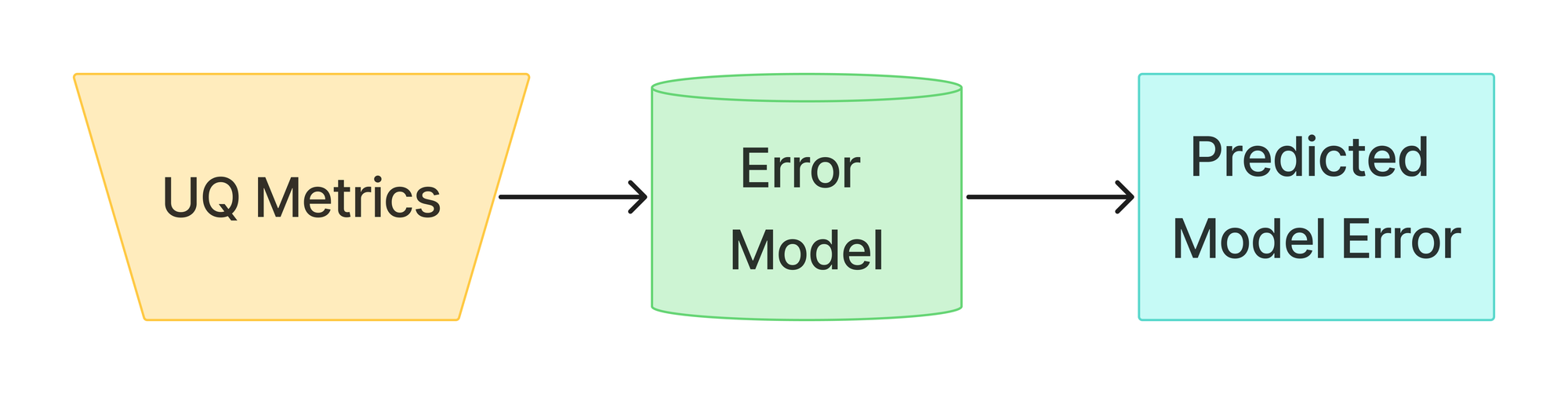
We primarily used UNIQUE to generate several error models with the pipeline’s built-in uncertainty quantification (UQ) metrics, see Table 2. Our computed Top-5 Tanimoto similarity and uncertainties were identical to those computed by the UNIQUE library for the top-5 Tanimoto similarity and ensemble variance. We also used the pipeline as a template to generate analogous error models trained on our baseline AD metrics described earlier. The main goal was to determine whether a combination of AD and UQ metrics, trained in an error model, showed a stronger correlation (ρ > 0.6) with ADME model error for specific endpoints than what we’ve seen with other metrics.

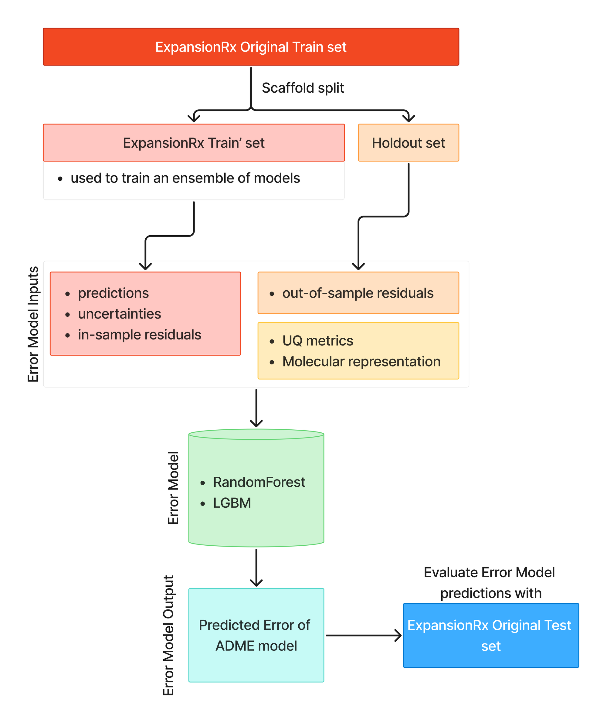
The full schematic for how we trained our error models is shown in Figure 7. In the UNIQUE pipeline, the error models are trained by splitting the data into three sets: train, holdout, and test. In this example using ExpansionRx data, we kept the original blind-challenge test set intact and split the training set into train′ and H using a scaffold-grouped split, with roughly 25% of Bemis-Murcko scaffolds held out. The train’ set is used to train an ensemble of models to generate prediction values and uncertainty. The ensemble model is then used for inference on the train’ set to generate in-sample residuals, which are optimistically low. For out-of-sample residuals, we use the ensemble model to predict on the holdout set.

The error model is fit on the combined train’ and holdout set, where the metrics described in Table 2 are the input features and the target is the absolute residuals. The error model is evaluated on the test set with the same 5x5 cross-validation previously shown.

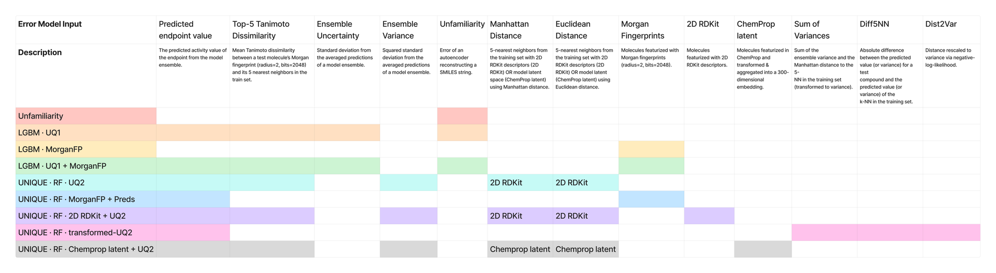
Figure 8 shows a matrix of the average Spearman’s ρ from 5x5 cross-validation for a selected subset of error models. As with the baseline AD metrics, we performed Tukey HSD comparisons to rank the best-correlated error model, outlined in dark blue. The error models that are tied in performance with the best are shaded with hashing. In these plots, we included the overall best single baseline AD metric, unfamiliarity, as a reference point. We can see that, with the exception of MGMB, which has a very small dataset, the best error model outperforms the single baseline AD metric. However, as we observed with the single-baseline AD metrics, no error model type ranks best across all endpoints.

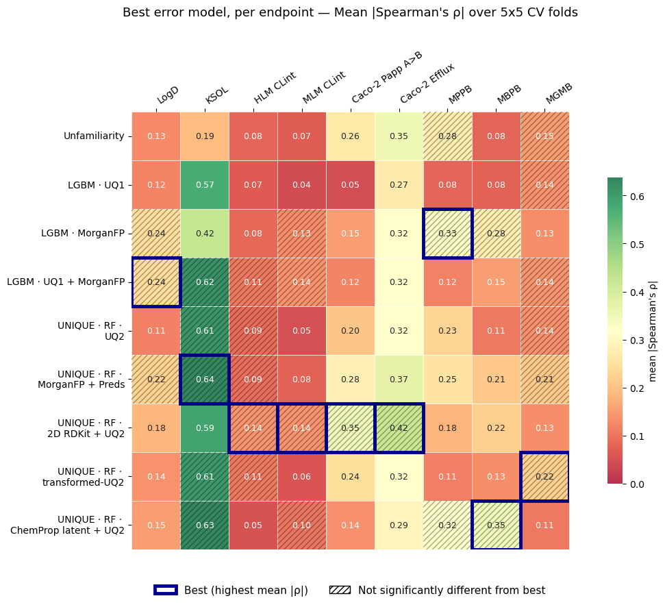
An interesting observation is that every top-ranked error model across all endpoints uses some kind of molecular representation as input, whether Morgan fingerprints or 2D RDKit descriptors. This shows the importance of calculating distance in some feature or latent model space rather than relying on a generic Tanimoto similarity. The UNIQUE RandomForest (RF) model, trained on 2D descriptors and UQ2 metrics (UNIQUE RF 2D RDKit + UQ2), is most strongly correlated with model error across four endpoints (HLM CLint, MLM CLint, Caco-2 Papp A>B, Caco-2 Efflux). Interestingly, for both Caco-2 endpoints, the UNIQUE RF 2D RDKit + UQ2 also outperforms the analogous UNIQUE RF ChemProp latent + UQ2 model, which differs only in that its Manhattan distance is calculated in latent space vs. descriptor space. This is curious because our ADME model actually uses the compound embeddings in the latent space to make property predictions.

Similarly, the best-performing error models for LogD and KSOL use Morgan fingerprints and prediction values, with no other UQ metrics as features. This implies that for some endpoints, an error model can learn something directly from a molecular representation that correlates with ADME model error. In addition to experimenting with various combinations of AD metrics, it may also be worth exploring different molecular representations as inputs to error models.

One important thing to keep in mind, however, is that although the error models clearly outperform the baseline UQ metrics in ranking model error, the correlations remain quite low overall (ρ < 0.6). The only exception is KSOL, which showed relatively high correlations even with the baseline AD metrics. These are the same trends that Parrando-Pizarro, R. et al. (2026) observed: while error models are certainly an improvement, they still fall short of providing actionable insights.

Conclusion

We have hopefully shown that defining AD is an extremely difficult and highly nuanced task that requires specific tailoring to your particular data set and the endpoints you’re looking at. There is no one-size-fits-all definition of AD, and anyone who claims otherwise is being delusionally optimistic.

That said, we confirmed the findings of Parrando-Pizarro, R. et al (2026) that error models are a very promising strategy for uncertainty quantification and defining AD. In particular, we find that it may be worth experimenting with different molecular representations as inputs to error models, since all of our best-performing error models across nearly all endpoints included some molecular featurization as direct input.

While these results may seem discouraging, they simply mean there is more room for innovation and improvement in this aspect of ADMET modeling. Stay tuned as we continue to run AD experiments!

Acknowledgements

We would like to thank our funders for their support of OpenADMET, in particular ARPAH, Radial (part of the Astera Institute (https://ror.org/00ydx1s47)), Schrödinger Inc, and the Gates Foundation.  We would also like to thank our partners Enamine, HuggingFace, OpenEye, CDD Vault, Discovery Life Sciences, and the beamline staff at NSLS-II for their support.

This work is supported by the Advanced Research Projects Agency for Health (ARPA-H) under AVOID-OME, and Award Number 1AY1AX000035. The contents are those of the authors. They may not reflect the policies of the Department of Health and Human Services or the U.S. government. The content is solely the responsibility of the authors and does not necessarily represent the official views of the Advanced Research Projects Agency for Health.