Peak Performance or Just Noise?

Statistical Comparison of Blind Challenge Entries
by Jon Swain
Benchmarks have become ubiquitous in machine learning, from the MNIST (Modified National Institute of Standards and Technology) dataset for computer vision to the SWE-bench leaderboard for LLM coding tasks. Benchmarks are standardized datasets or tasks used to evaluate models, comparing metrics such as performance, reproducibility, and efficiency for domain specific tasks.
Blind challenges, a specialized, high-rigor subset of benchmarks where the ground truth is withheld until the end of the challenge (or even generated prospectively), are emerging as the gold standard in benchmarking, reducing data leakage and overfitting associated with open leaderboards. Blind challenges such as CASP (Critical Assessment of Protein Structure Prediction) have done more than just track progress; they have actively driven it, providing the rigorous environment necessary for breakthroughs like AlphaFold. The best blind challenges turn a fragmented research field into a collective, community-focused, yet still competitive sprint, standardizing how success is measured.
OpenADMET is an international open-science initiative dedicated to transforming predictive modeling in drug discovery by generating high-quality, standardized experimental datasets. By integrating rigorous ADMET assays with detailed structural data, the initiative addresses the critical data gaps that often hinder the accuracy of machine learning models. These efforts are put into practice through a series of blind challenges, including the recent ASAP Polaris OpenADMET Challenge and the OpenADMET ExpansionRx Blind Challenge, both of which featured data derived from actual drug discovery programs. Furthermore, the current PXR Challenge uses data from internally developed and run high-quality assays, ensuring consistency and precision often lacking in public repositories. By hosting these competitions, OpenADMET provides a transparent benchmarking environment that drives the field forward, establishing new performance standards and identifying robust methodologies for navigating the complexities of the "Avoid-ome”.
However, even the best benchmarks become saturated over time, with apparent performance improvements due to hyper-specialized overfitting (i.e., benchmark-hacking) and not genuine improvements in the model's performance. This creates a translation gap where a model wins on a technicality but fails in the real world. The traditional way we crown a winner, by simply sorting by a performance metric, is a fragile approach. It treats a leaderboard as a definitive ranking rather than a noisy snapshot. To justify real-world decisions and significant lab resources, we need to move beyond raw scores and determine if the "best" model is actually, statistically, the best.
When first place is just a rounding error
Blind challenges with newly created test datasets solve or reduce overfitting and leaderboard saturation, especially with limited entries, but a perfectly designed blind leaderboard is still just a single snapshot in time. To truly crown a champion, we need to account for the inherent noise in the system by performing rigorous statistical analysis of model performance.
Static leaderboards typically have three main issues:
-
A model may appear to win simply due to a fortunate random seed or a specific initialization that happened to align with the test set's distribution. Without statistical testing, we risk rewarding a lucky participant, rather than a robust architecture.
-
In chemistry, a pair of molecules with an activity cliff can disproportionately skew performance metrics. If a model’s lead is brittle, it might vanish if just one or two tricky molecules are removed from the set. Statistical rigour helps us measure the stability of a model's performance across the entire chemical space.
-
In many cases, the margin between places on a leaderboard is smaller than the assay's experimental uncertainty. If the physical measurements are only accurate to ±0.3 log units, claiming a winner based on a 0.01 difference in MAE is mathematically suspicious.
When models are statistically indistinguishable, decisions may be made based on secondary metrics such as inference time, cost (open-source vs. proprietary APIs), and model explainability.
To guide real-world decision-making, an ideal statistical framework must do two things:
- Perform signal-to-noise separation. Is a model truly superior, or did they get lucky?
- Quantify lead stability. Is the lead robust, or would changing the dataset change the performance gap?
Comparing machine learning models
Statistically sound methods for comparing machine learning models are an ongoing area of research. “Practically Significant Method Comparison Protocols for Machine Learning in Small Molecule Drug Discovery” proposes a set of rigorous guidelines for method comparison in this field.
The authors suggest a nested 5x5 cross-validation strategy:
- Generate 25 different models using the same architecture but with different random seeds and data folds.
- Use these 25 models to generate a distribution of scores on a consistent test set.
- Compare these distributions using ANOVA to determine if there is a statistically significant difference in performance
- Use Tukey’s Honestly Significant Difference (HSD) test for post hoc pairwise comparisons. The Tukey HSD test controls for the Family-Wise Error Rate (FWER), the increase in Type I errors due to repeated pairwise comparisons.
Whilst this method works well for comparing new machine learning methods, it is not practical to use it for a blind challenge. It would create a significant submission burden for participants, who would be required to submit 25 sets of predictions. It also leaves the leaderboard susceptible to gaming, as unscrupulous participants could submit one set of predictions with minimal noise added to simulate a distribution.
An alternative would be to ask participants to submit their training code, and have the challenge backend train the models and make predictions. This would require training 25 versions of every entry, a massive computational expense. Additionally, many participants use proprietary datasets or architectures. They are often happy to share their final predictions but are understandably reluctant to hand over their source code or weights.
Because we cannot change the models, we have to change how we look at the data. We need a method that can extract robust statistics from a single set of predictions.
The ExpansionRx blind challenge
The OpenADMET-ExpansionRX blind challenge wrapped up in January 2026. Thank you to everyone who took part, and congratulations to our winners!
Crowning a champion
This was our first attempt at including a statistical comparison of entries, and we adapted the methodology from the above paper for a static blind challenge. The primary metric used was the Macro-Average Relative Absolute Error (MA-RAE). The RAE was chosen over the Mean Absolute Error (MAE) to account for the challenge's multiple endpoints with different absolute scales, which were averaged to compute a single metric.
To generate a distribution of the performance metric for each entry, pseudo-test sets were generated by sampling with replacement (bootstrapping) from the test dataset. This is a common approach for estimating the variance of population-level statistics via resampling, and is perfect for situations like this where only a single set of entries is available. These pseudo-test sets were the same size as the static test dataset and used the same sampling for each entry. This was repeated for 1,000 bootstrap iterations (a common choice), and the MA-RAE was calculated each time. The performance metrics from the 1,000 bootstrap iterations were treated as a performance distribution, and Tukey’s HSD test was used to determine statistical significance, which was represented by the Compact Letter Display (CLD) on the leaderboard.
Manufacturing evidence: Creating data out of nothing
Whilst this was a good attempt at a robust statistical comparison of entries, it had some major limitations that we raised at the time. Bootstrapping to create test datasets involves sampling from the same molecules, creating the illusion of more data through pseudoreplication. These bootstrapped samples are independent in the sense that the creation of one bootstrap sample does not affect the next, but the samples are highly correlated to the original population, and therefore to each other. This likely underestimates the variance in model performance.
The HSD formula calculates the minimum difference between two means necessary to be considered statistically significant. It is defined as:
$$\mathrm{HSD} = q_{α,k,df} \sqrt{\frac{\mathrm{MS_{Error}}}{n}}$$
Where:
$q_{α,k,df}$ = The standardized range statistic, which depends on the significance level ($α$), number of groups ($k$), and the degrees of freedom ($df = N - k$, where $N$ is the total number of observations)
$MS_{Error}$ = The mean square error for within groups from the ANOVA
$n$ = The number of observations per group
The number of bootstrap iterations will affect both the number of observations per group (n), and the total number of observations (N). Increasing the number of bootstrap iterations will reduce the standard error term to near zero, shrinking the confidence intervals and leading to an overpowered test. This leads to a situation where it is possible to produce a desired outcome of the statistical test by changing a hyperparameter, here the number of bootstrap iterations, known as p-hacking. Whilst 1,000 bootstrap samples is considered standard, it is still a slightly arbitrary default.
To clarify, whilst it requires some compromises, using a 5x5 CV approach followed by ANOVA and Tukey’s HSD test is a statistically valid method for comparing machine learning models. The issue here lies in using this method for comparing a large number of bootstrapped samples. When using 5x5 CV, n is 25 (the number of models), but here n is the number of bootstrap iterations. We’re effectively telling the statistical test that we have 1,000 independent test datasets, whereas we really have one model and one test set that is being resampled. This leads to the observed p-value collapse.
This effect is demonstrated in Figure 1. The predictions for the top 10 participants in the ExpansionRx challenge for predicting LogD were assessed using the Tukey HSD test on bootstrapped samples, with the number of bootstrap iterations ranging from 10 to 1,000.1 With a low number of bootstrap iterations, there is significant overlap in the confidence intervals between most entries. As the number of bootstrap iterations increases, the confidence intervals shrink, and by 1,000 bootstrap iterations, the performance of almost all entries is considered statistically different. Across the entire range of bootstrap iterations, pebble’s entry remains at the top of the leaderboard, statistically different from any other entry (congratulations, pebble!).
With regard to the ExpansionRx challenge, we want to emphasise that the rankings themselves stand. However, our analysis of which leaderboard entries are statistically distinct is likely overpowered.

The key difference here is that 5x5 CV measures epistemic uncertainty (model stability), i.e., how much does the model performance change if it is trained differently? Whereas the bootstrap measures aleatoric uncertainty (data stability) on a fixed test set, i.e., how does the performance change if the test set changes?
Since the bootstrap and Tukey approach leads to over-confident rankings and is susceptible to p-hacking, we need a framework that respects the limits of our data.
Head-to-head bootstrap comparisons
Whilst bootstrapping followed by Tukey’s HSD leads to over-confident rankings, bootstrapping does give us useful information about how a model would perform on different test sets, and can be analysed in different ways. One method is using Paired Bootstrap Confidence Intervals, based on the resampling methods developed by Bradley Efron.
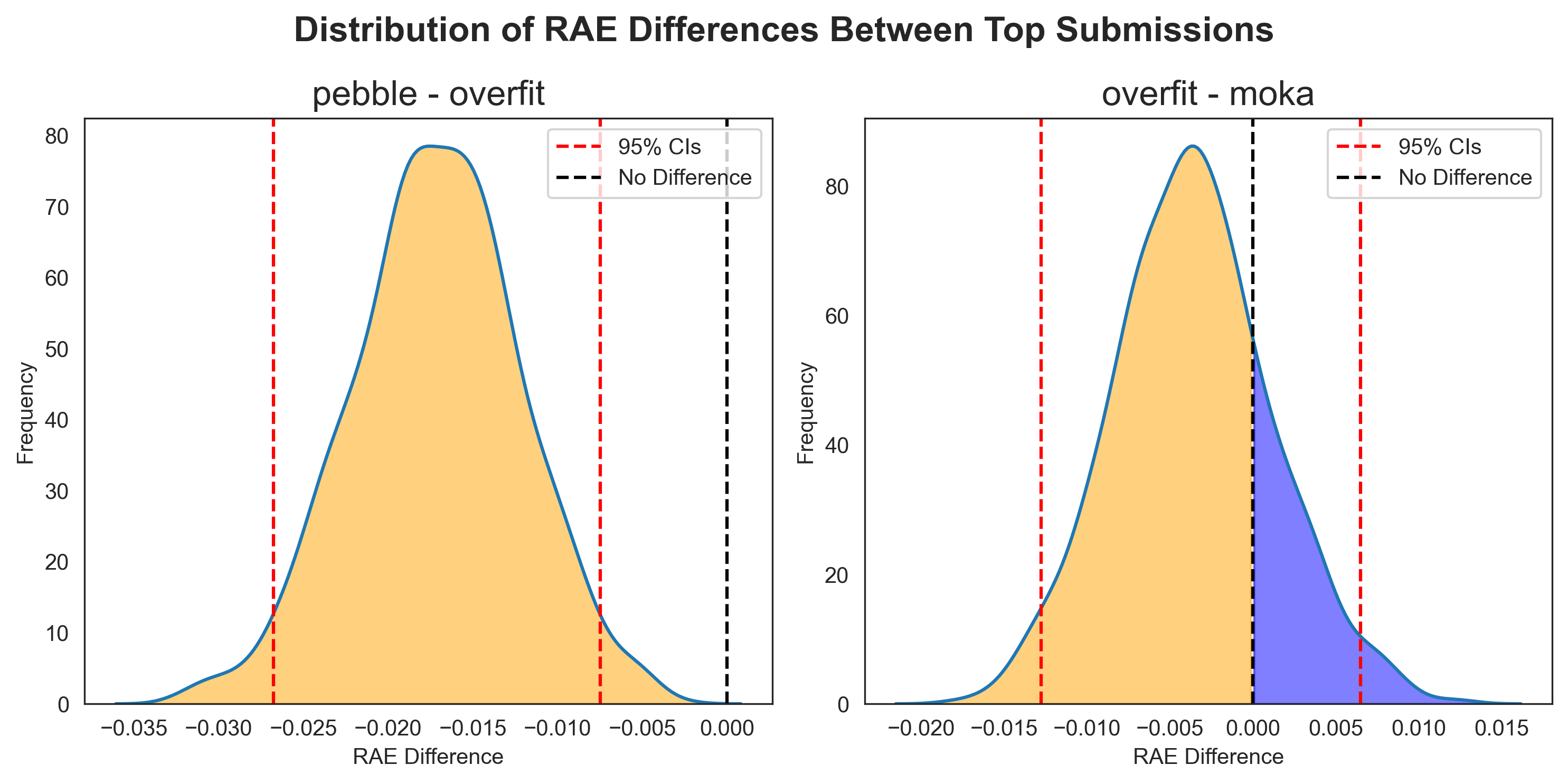
Since each bootstrap iteration uses the same samples for each user, we can directly compare participants' performance. If we select a pair of entries and, for each bootstrap sample, subtract the score for one participant from the other, we can generate a distribution of the performance differences, ΔRAE (Figure 2). Instead of treating bootstrap samples as new data points for a ranking test, we use them to see how two models perform head-to-head under varying conditions.
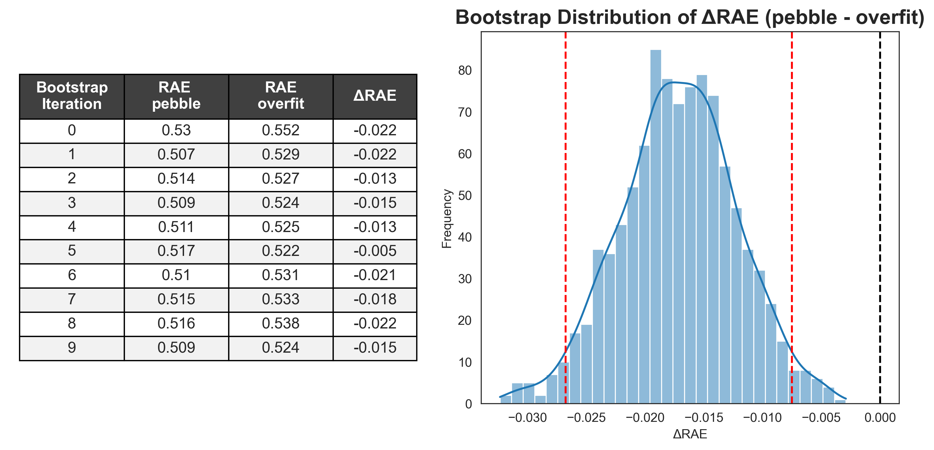
With a distribution of the difference in performance across a large number of pseudo-test sets, we can now calculate the 95% confidence intervals from the 2.5 and 97.5 quantiles.2 The 95% confidence interval represents the range of values that would encompass the true difference in 95% of repeated experiments.
This method was applied retrospectively to the top three participants from our ExpansionRx challenge (“pebble”, “overfit”, and “moka”). All three entries were considered statistically different when (improperly) using the Tukey HSD test.
Across the 1,000 paired bootstrap iterations, pebble outperformed overfit each time (Figure 3, left). The null hypothesis (that there is no difference in performance between pebble and overfit, where ΔRAE = 0) falls well outside the 95% confidence intervals calculated from the distribution. We can say with 95% confidence that there is a statistically significant difference in performance between the two entries.
When comparing overfit and moka, whilst overfit sat one place higher on the leaderboard, moka actually had a higher performance in 211 of the 1,000 bootstrap iterations (Figure 3, right), making it difficult to argue that we are 95% confident that these entries have statistically different performances. To put it another way, we simulated the performance of the models on test data 1,000 times, and moka was better in 21.1% of these simulations. The null hypothesis falls within our 95% confidence interval, so we cannot reject it.
Stability in 1-to-1 comparisons
Using paired bootstrap confidence intervals has some big advantages. Unlike the Tukey test, it is robust to the number of bootstrap iterations; adding more iterations here only improves the resolution of the distribution; it doesn’t artificially shrink the width of the confidence interval. It makes no assumptions about the distribution of the difference in performance, making it a non-parametric test.
By pairing the bootstrap iterations, we account for the inherent difficulty of each bootstrapped pseudo-test set. If a specific resample contains a cluster of difficult activity cliffs, both models' performance will likely drop. However, the difference (ΔRAE) between them remains a pure measure of relative skill.
Too much of a good thing
Paired bootstrap confidence intervals are ideal for head-to-head comparisons, but they don’t have a built-in control for multiple comparisons. If our leaderboard has 100 participants, we have to complete nearly 5,000 (100 x 99 x 0.5) pairwise comparisons, and at a 95% confidence interval, that leaves a lot of room for Type I (false positive) errors, and risks increasing the Family-Wise Error Rate (FWER).3
One method for controlling the FWER is the Bonferroni correction. A new, stricter significance level (α) is calculated by dividing the original α by the number of comparisons. This is a very conservative method. With an example leaderboard with 100 participants, we must complete 4,950 comparisons, which would shrink our α to 1 x10⁻⁵. In this situation, even if we bootstrapped 100,000 times and one participant wins for 99,999 of the bootstrap samples, we would not see a significant difference. This could lead to significant Type II (false negative) errors.
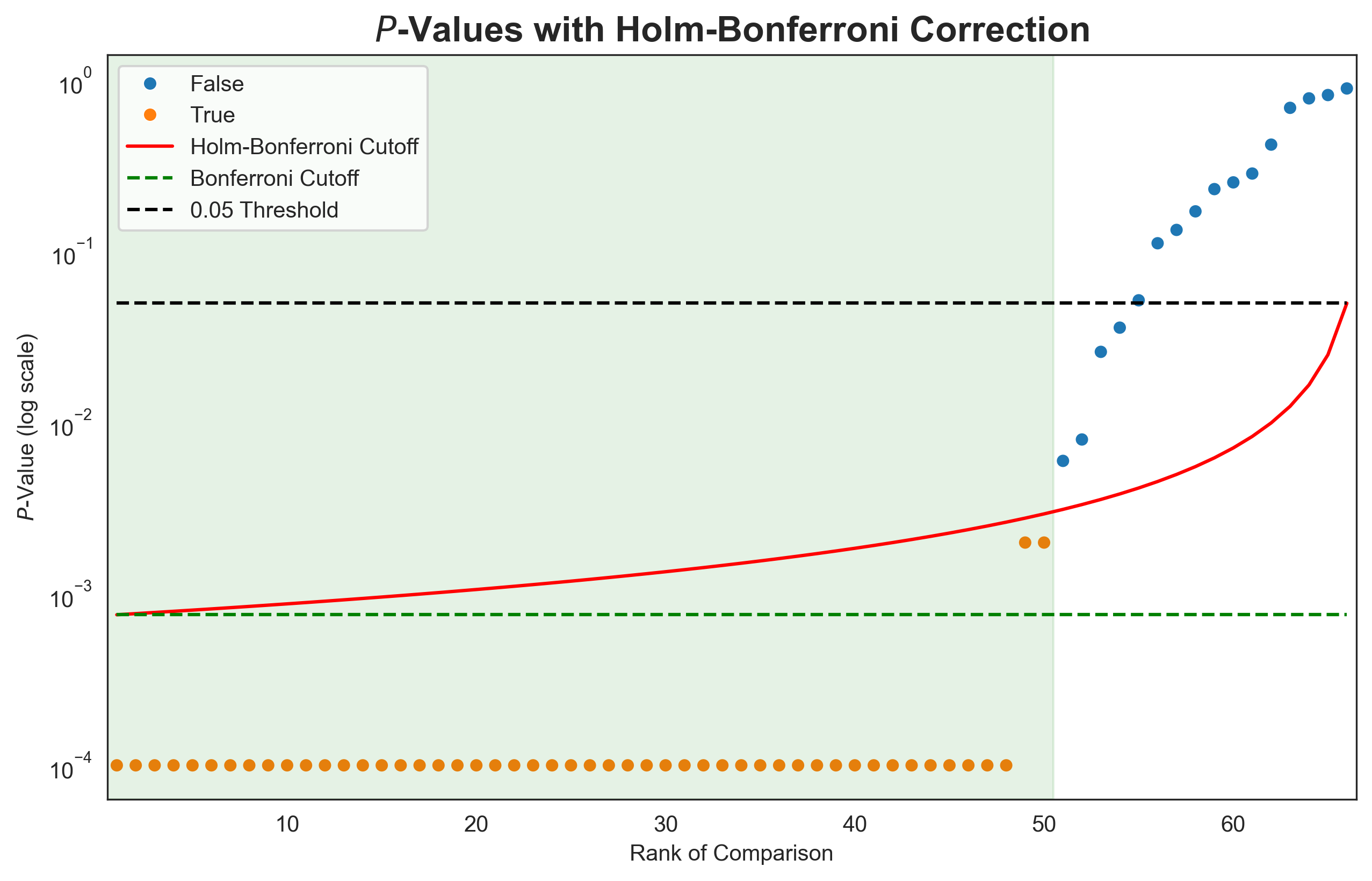
Whilst the Bonferroni correction is a sledgehammer, a less aggressive adaptation, the Holm-Bonferroni method, retains more of the power of the statistical test. Using this method, the p-values for m pairwise tests are sorted in ascending order. The first p-value is compared to the Bonferroni corrected α (α/m), the second to α/(m-1), continuing until the mth p-value is compared to the original α (the significance level). If the p-value is below the comparison α, the null hypothesis is rejected, and a significant difference is observed. If the p-value is above the comparison α, we cannot reject the null hypothesis for that comparison, or any subsequent comparisons, even if the p-values fall back below the rising Holm-Bonferroni adjusted α. This is demonstrated in Figure 4 for the top 12 entries from our ExpansionRx challenge. P-values were calculated as the proportion of bootstrap iterations where the lower-ranked entry achieved a higher performance, and pairwise comparisons between 12 entries yielded 66 p-values. For 48 out of 66 comparisons, the higher placed entry performed better across all bootstrap iterations, yielding p-values of 0.4 As the p-value rank increases, the p-values eventually cross the Holm-Bonferroni cutoff, and all further comparisons have no significant difference.
Head-to-head comparisons on the ExpansionRx leaderboard
Using the Paired Bootstrap Confidence Intervals with the Holm-Bonferroni method to control for multiple comparisons, we can regenerate the CLD for our top 12 entries to the ExpansionRx challenge.
| Rank | User | MA-RAE | Original CLD | New CLD |
|---|---|---|---|---|
| 1 | pebble | 0.5113 ± 0.0070 | a | a |
| 2 | overfit | 0.5284 ± 0.0070 | b | b |
| 3 | moka | 0.5321 ± 0.0070 | c | b |
| 4 | campfire-capillary | 0.5517 ± 0.0069 | d | c |
| 5 | shin-chan | 0.5536 ± 0.0073 | e | c,d |
| 6 | HybridADMET | 0.5582 ± 0.0072 | f | c,d |
| 7 | rced_nvx | 0.5663 ± 0.0073 | g | d,e |
| 8 | tibo | 0.5672 ± 0.0073 | g | d,e |
| 9 | beetroot | 0.5726 ± 0.0075 | h | e,f |
| 10 | temal | 0.5809 ± 0.0074 | i | f,g |
| 11 | yanyn | 0.5818 ± 0.0071 | i | f,g |
| 12 | crh201 | 0.5824 ± 0.0079 | i | g |
Whilst these adjustments will reduce the FWER, we could also consider using a method with built-in control for multiple comparisons, similar to Tukey's HSD test.
Shuffling the deck: Permutation testing
When comparing entries, we want to know if we can reject the null hypothesis: “There is no statistically significant difference between the entries”. One way to do this is to simulate the null hypothesis through Permutation Testing. If there is no significant difference between the entries, we should be able to swap their predictions without significantly changing the measured performance.
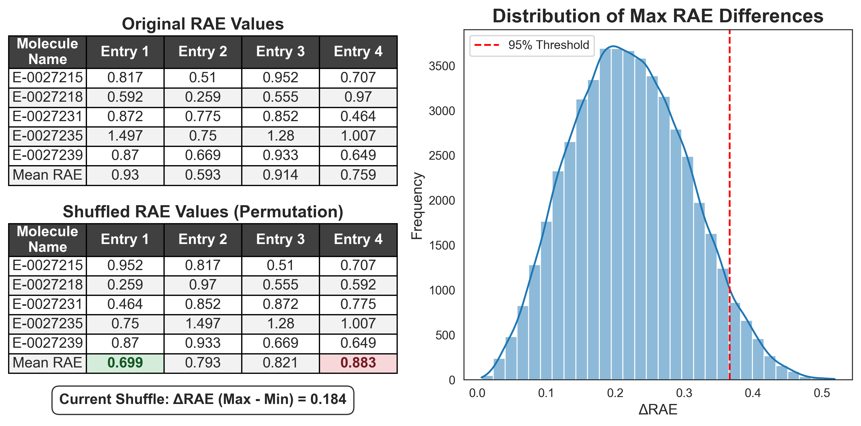
For our leaderboard, we would first calculate the performance of entries on the entire test set and use permutation testing to determine whether these performances are sufficiently different to be considered statistically significant. We first gather the RAE values for each entry for each molecule in the test set. This data is stored in a table with one column for each entry, and each row represents one molecule from the test set. The table is populated with the RAE values.
During each permutation test, the RAE values are randomly shuffled across the row, so that the RAE values remain associated with the corresponding molecule, but are found under a random entry (Figure 5). These randomised entries are scored, and the largest difference in performance between two entries is recorded. This is repeated many times (for example, 1,000 permutations), building a distribution of the largest observed performance difference from randomly shuffled entries. We can take the 95th percentile of this distribution to define a threshold, above which the difference between entries exceeds 95% of those observed by chance; i.e., the difference is statistically significant.
By recording only the maximum difference observed across the entire leaderboard in each shuffle, we build a distribution of the “biggest fluke”. This distribution tells us how large a performance gap can be driven by pure luck among participants. We then take the 95th percentile of these maximum flukes to set a single, global threshold. To be considered statistically significant, a real-world lead must be larger than this “best-case luck” threshold.
One threshold to rule them all
Using the raw difference to set a global threshold is simple and intuitive, but it relies on the entries having consistent variance. It can be very sensitive to outliers, where a single entry with wildly inconsistent performance (high variance) can inflate the global threshold, making it difficult for more consistent entries to prove significance.
An extension of permutation testing is the Westfall-Young Step-Down (or Westfall-Young Max-t) test. This method still shuffles labels row-wise, but instead of calculating the raw difference between performance metrics, it computes the paired t-statistic for each pair of entries and records the maximum t-value observed by chance. The 95th percentile maximum t-value is used as a threshold for pairwise comparisons, and pairs of entries with a t-value greater than this threshold are considered statistically different.
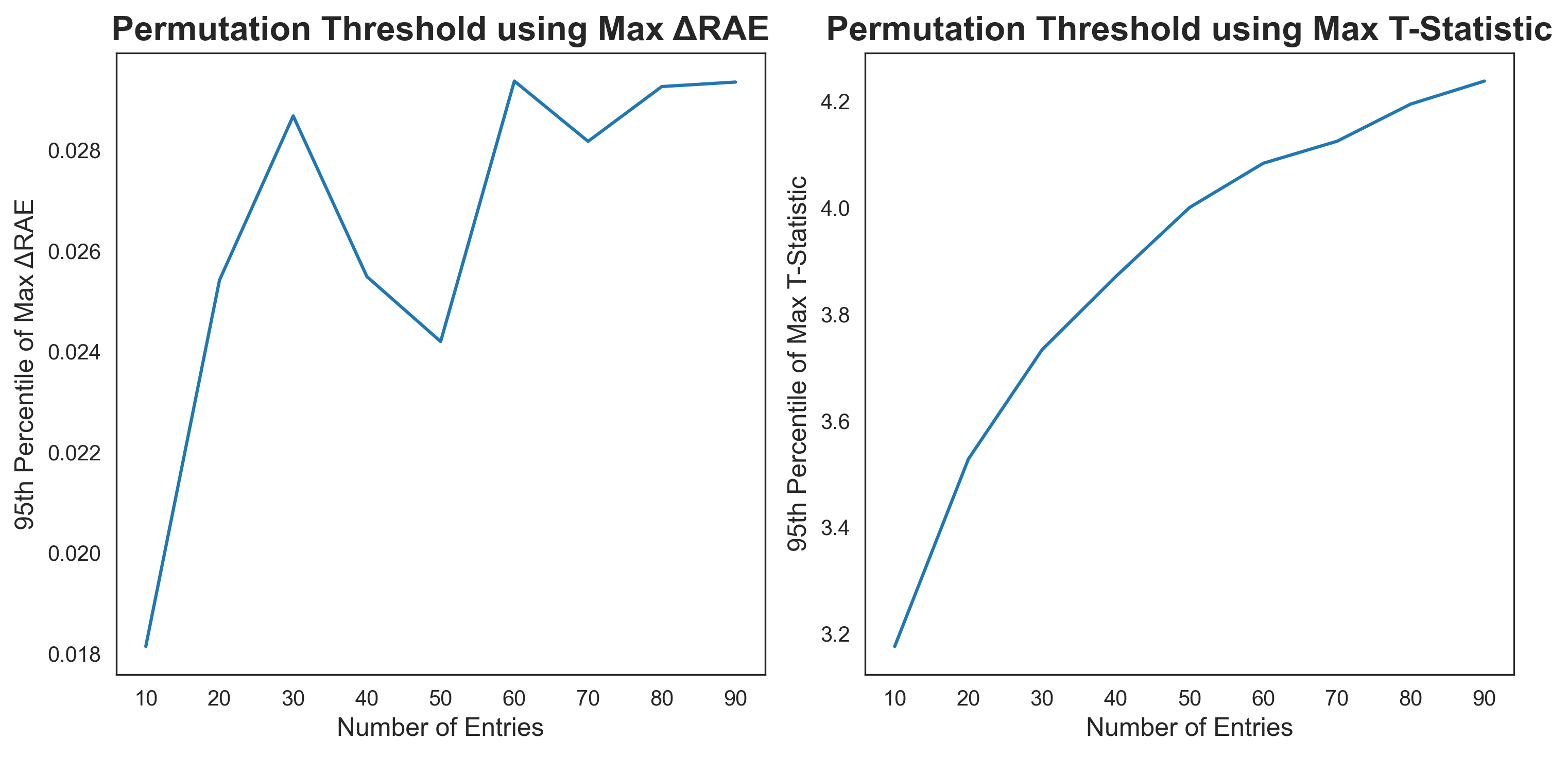
Both methods intrinsically control the Type I error rate as the number of comparisons increases. As the number of entries increases, the chance of an extremely high or low combination of predictions increases. By taking subsets of entries from the ExpansionRx challenge and calculating a permutation threshold using both methods, we observe that the threshold increases with the number of entries (Figure 6). The threshold calculated using the maximum ΔRAE is very sensitive to the selection of entries, and one entry with lots of poor predictions can make a big difference. The threshold calculated using the maximum t-statistic has a much smoother increase as the number of entries increases.
Finding truth in the scramble
The primary appeal of permutation testing lies in its extreme intuition. Unlike abstract p-value corrections, the logic here is transparent: if we scramble the labels 10,000 times and the real-world lead is still larger than the best "fluke" lead, we can be confident the difference in performance is real. This is particularly effective with the Raw Difference method, as the resulting threshold is expressed in the same units (RAE) as the leaderboard.
Similar to the paired bootstrap method, permutation testing makes no assumptions about the underlying distribution of your data (a non-parametric method). Furthermore, because the null distribution is built from the ground truth of the dataset, it remains insensitive to the number of bootstrap iterations used in previous steps.
Most importantly, it provides a built-in control for multiple tests by naturally raising the bar as more entries are considered, ensuring that the Type I error rate is controlled.
Lost in the shuffle
Whilst permutation testing offers a robust way to determine whether two models have statistically different performance, it doesn’t provide a good measure of lead stability, since it uses the entire test set for each test. It doesn't tell you if Entry A beats Entry B because of a few lucky molecules or consistent superiority across the whole chemical space. It can also be very sensitive to outliers; if a few entries have particularly bad predictions or particularly high variance, it can lead to an inflated threshold for every entry.
An interesting quirk of the max-t-value permutation test is that results can produce non-contiguous groupings. In a situation with three ranked entries, A, B, and C, where A and C have large variances, but B has a small variance, you could find a situation where A and C are considered not statistically different, but A and B, and B and C are considered statistically different, making leaderboards look counterintuitive.
Permutation testing in practice
Using both Permutation Testing methods to determine thresholds for statistically significant differences between entries, we can again regenerate the CLD for our top 12 entries in the ExpansionRx challenge. The calculated 95th percentile ΔRAE threshold was 0.017, and the t-statistic threshold was 3.27. While there is a slight shuffle in the leaderboard order due to evaluating the entries on the entire static test set rather than on individual bootstrap samples, this shift provides evidence that the differences among many of these models are statistically negligible. However, it is important to note that while permutation testing offers a method to determine differences in performance between entries, it provides no inherent measure of the variance for the MA-RAE metric itself, an insight that remains exclusive to the bootstrapping approach.
| Rank | User | MA-RAE | Max ΔRAE CLD | Max t-statistic CLD |
|---|---|---|---|---|
| 1 | pebble | 0.509 | a | a |
| 2 | overfit | 0.534 | b | b |
| 3 | moka | 0.535 | b | b |
| 4 | campfire-capillary | 0.560 | c | c,d |
| 5 | shin-chan | 0.562 | c | c,d |
| 6 | rced_nvx | 0.562 | c | c,d |
| 7 | beetroot | 0.565 | c | c* |
| 8 | crh201 | 0.572 | c | d,e,f* |
| 9 | HybridADMET | 0.574 | c,d | c,d,e,g* |
| 10 | Gashaw | 0.590 | d,e | e,f,g,h |
| 11 | yanyn | 0.591 | d,e | f,h* |
| 12 | tmp1234 | 0.592 | e | g,h* |
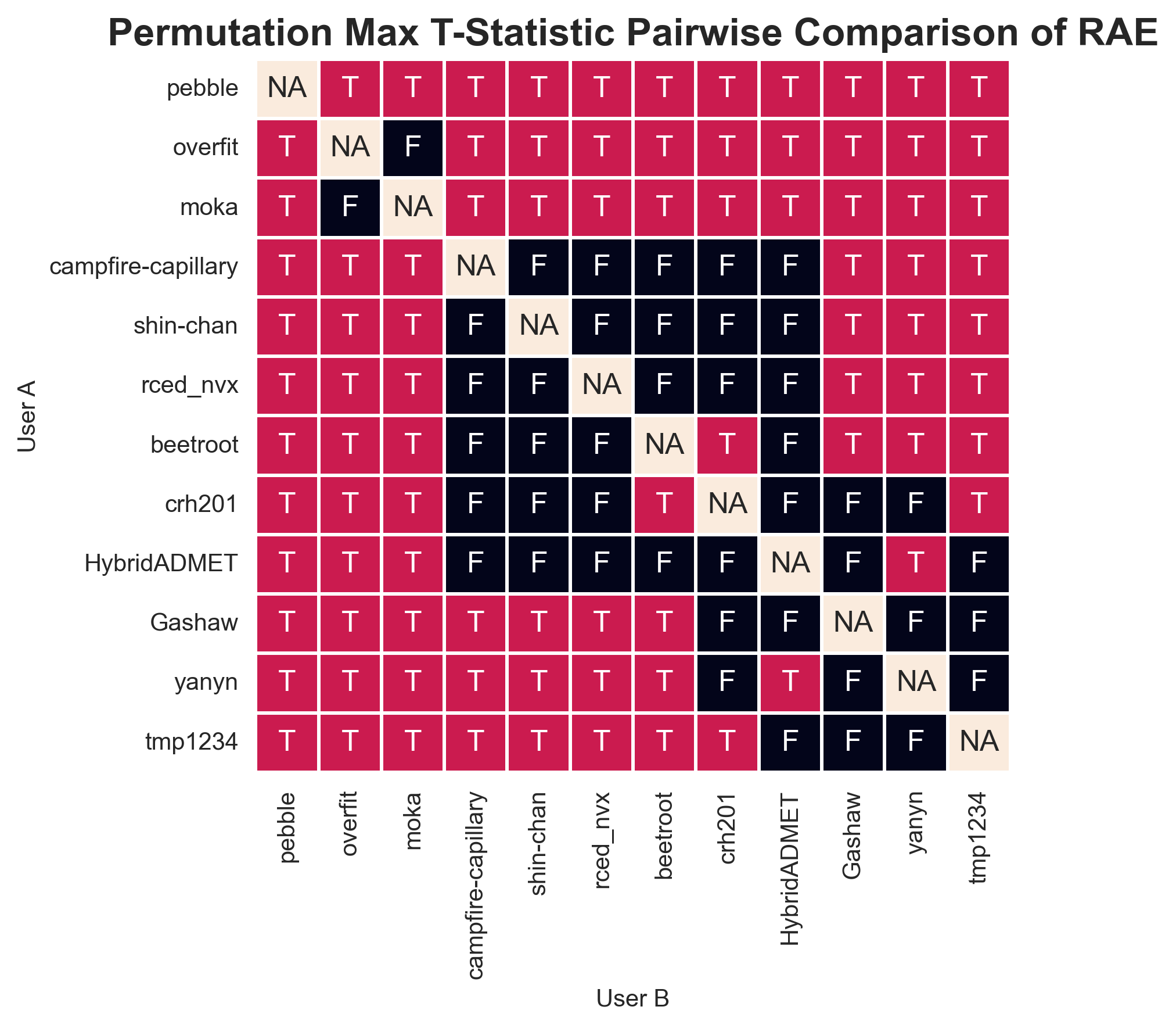
As you can see from the table, the Max t-statistic method can make the Compact Letter Display less compact, turning it into alphabet soup. Entries marked with an asterisk are part of complex, non-contiguous groups. For a small leaderboard, this can be more easily represented using a pairwise “battle-map” (Figure 7). This offers a clear representation of the pairwise comparisons for a small group of entries, but it would not be possible for an entire leaderboard.
The final showdown: Comparing the methods
To wrap things up, let's look at how these four methods stack up across four key categories: their mathematical assumptions, their sensitivity to the number of simulations, their greatest strength, and their biggest flaw.
Bootstrap plus Tukey’s HSD test
- Assumptions: Parametric. Assumes normal distributions and relies on ANOVA's Mean Square Error.
- Sensitivity: High. More bootstrap iterations artificially shrink the confidence intervals, increasing the risk of accidental p-hacking.
- Strengths: Familiar, standard, and easy to run straight out of a Python library.
- Weaknesses: Mathematically suspicious for this use case. It treats reshuffled data as brand-new, independent information, leading to wildly overconfident rankings. Pseudoreplication alert!
Paired bootstrap confidence intervals
- Assumptions: Non-parametric. Makes zero assumptions about the underlying distribution of the performance gap.
- Sensitivity: Low. Increasing the number of iterations just gives you a higher-resolution picture of the true distribution; it doesn't artificially shrink the confidence intervals.
- Strengths: Measures total performance and lead stability. It is an intuitive method that successfully cancels out the "difficult sample" factor.
- Weaknesses: The multiple comparisons problem. Requires methods to control the Family-Wise Error Rate (FWER), like Holm-Bonferroni, which can reduce statistical power.
Max ΔRAE permutation
- Assumptions: Non-parametric. Built purely from the ground truth of the existing dataset.
- Sensitivity: Low. Shuffling 10,000 times just helps define the "luck threshold" more accurately.
- Strengths: Deeply intuitive. It outputs a global threshold in the exact same units as the leaderboard (e.g., RAE) and inherently controls for multiple comparisons.
- Weaknesses: A single high-variance entry can inflate the global threshold. Furthermore, it only measures total performance, not lead stability.
Max t-statistic permutation
- Assumptions: Partially parametric. While the permutation itself is non-parametric, it relies on calculating a t-statistic, which standardizes by variance.
- Sensitivity: Low. Shuffling 10,000 times just helps define the "luck threshold" more accurately.
- Strengths: Controls the FWER without being hijacked by a single noisy outlier, providing a highly robust threshold. Scales smoothly and elegantly as you add more entries to the leaderboard.
- Weaknesses: Can generate counter-intuitive leaderboards, with non-contiguous groups where Model A and C are tied, but Model B sits awkwardly between them.
So, which one should I use?
After careful comparison and consideration, the Paired Bootstrap Confidence Intervals with Holm-Bonferroni correction emerge as a winner.
The intuitive nature of paired bootstrap confidence intervals makes the method ideal for our use-case. Put simply, it can be explained as “We simulated a head-to-head comparison between these two entries 1,000 times, and Entry A won over 95% of the time.”
By pairing the models up on the exact same bootstrapped test sets, it completely cancels out the sampling noise. If a resample pulls the most brutal, uncooperative molecules from the dataset, both models suffer equally. The only thing left to measure is pure, relative skill.
It also measures actual stability, not just peak performance. Unlike permutation tests that only look at the final macro-score, the paired bootstrap focuses on consistency. It tells us if a model is genuinely better across the chemical space of the test dataset, or if it just got lucky on a handful of weird molecules.
Importantly, it appears to work in the real world. Empirically, when looking at our ExpansionRx dataset, this method produced the most justifiable rankings. It separated the true signal from the noise without generating bizarre, non-contiguous tiers (looking at you, Max-t Permutation).
Paying a 'Holm-Bonferroni tax' to control the Family-Wise Error Rate reduces the statistical power and makes it harder to prove a definitive winner. But in the world of drug discovery, where crowning a false champion costs real time and lab resources, setting a high bar can be a good idea.
- Some examples in this blog post measure performance using the RAE, whereas others use MAE. Where the original bootstrap data could be used, entries are compared using the RAE to match the original ExpansionRx challenge leaderboard. For some simple examples, the MAE for just the LogD prediction task is used to compare entries to reduce having to recalculate the MA-RAE across multiple endpoints. ↩
- This is a two-tailed test that determines whether the null hypothesis (ΔRAE=0) falls outside the 95% confidence interval. While a one-tailed test would specifically test the directional hypothesis: “Entry A outperforms Entry B”, it requires the direction to be specified before the data is seen. Since we do not know the relative performance of participants when designing the benchmark, choosing a one-tailed test after viewing the leaderboard would constitute HARKing (Hypothesizing After the Results are Known), an example of p-hacking. ↩
- The Family-Wise Error Rate (FWER) is the probability of making even one single False Positive across the entire leaderboard. This is different to the False Discovery Rate (FDR), the proportion of False Positives among all significant results. If there are 100 significant findings and an FDR of 0.05, 5 of them are expected to be due to random chance. ↩
- With 1,000 bootstrap iterations, the empirical resolution of our p-value is limited to p < 0.001 (1/number of bootstrap iterations). However, because the higher-ranked entry outperformed the lower-ranked entry on every single molecule in the original test set, there is no possible combination of resamples where the ranking could flip. Because of this we can claim p-values of 0, from a theoretical infinite number of bootstrap iterations. ↩