Authors: Devany West and Jackson Burns

What is foundational training?

It is a well-known issue that cheminformatics and machine learning models struggle to predict properties of compounds outside the chemical space they were trained on. Meanwhile, over the last few years, we’ve seen the rise of large-language models (LLMs) that exhibit incredible emergent properties and an uncanny ability to extrapolate from training data. Of course, this is largely due to the massive amount of data used to train these models, with dataset sizes in the trillions. 

For us cheminformaticians, public assay datasets are many, many orders of magnitude smaller, frequently fewer than 1000 compounds. Even in industry settings, cheminformaticians are working with a paltry few million datapoints, and all of that data is extremely expensive and time-consuming to collect. Searching for an LLM-esque breakthrough in these conditions can feel disheartening, and it’s hard not to peer over the fence at the LLM builders and quietly seethe at their wealth of data. But part of our job as scrappy cheminformaticians is to find crafty ways to improve our model performance with what we’ve got! One of these clever methods, developed to achieve deeper chemical understanding, is foundational training. 

Foundational training for cheminformatics makes use of the fact that, though experiments are expensive to run, there are countless in-silico featurization strategies that allow us to precompute information about our compounds of interest. Some common examples include molecular fingerprints (e.g., Morgan fingerprints), molecular descriptors (e.g., the 200+ RDKit descriptors), and properties from quantum-mechanics calculations. While these properties are often fed into our models as features, they can also serve as training targets. This is useful because it means we can rapidly and at very little cost create large, general chemical datasets on which to train models. 

Foundational training then proceeds in two steps: we perform an initial training run (pretraining) on a large, computed dataset. After pretraining, we initialize a new network using the weights from our pretrained model. Then, we attach a new, randomly initialized network for final prediction, and train again on a smaller, targeted dataset for a specific task (which we refer to as fine-tuning). In theory, our pretrained weights carry representational and chemical information that could correlate with endpoints of interest. However, it is unclear whether this approach works because these weights carry general chemistry information that won’t emerge from a smaller dataset, or whether the weights simply allow for a “hot start,” helping the network learn more quickly and efficiently. We will speculate about this later, but definitive evidence for either theory is beyond the scope of this humble blog post.

Though the exact “how” of foundational training is still a mystery, it is a proven approach. Many industry groups use their own internal pretrained models for property prediction, and in our blind challenges, pretraining on supplemental data was one of the most effective ways to improve performance (see the ExpansionRx and PXR results). Despite their prevalence, there has been little public work on the various parameters of foundational training (pretraining dataset size, chemical space coverage, featurization scheme, etc.), and their influence on performance. Often, it is possible for groups to achieve improved performance by throwing everything they have at a given model, whether that be by massively multitasking on all available data or ensembling models into one Frankenstein’s monster of a meta model. Systematic approaches are less common, though not unheard of (see here and here). At OpenADMET, we wanted to understand the impact of foundational training on model performance in more fine-grained detail.

To investigate this, we chose to run an extensive series of experiments on training foundation models. According to our blind challenges, there are a few standout architectures. The Directed-Message Passing Neural Network (D-MPNN) implemented in Chemprop, and in particular the Chemprop-based foundation model CheMeleon, an architecture pretrained on a set of one million molecules with Mordred descriptors, were very popular choices. Therefore, we decided to make CheMeleon the subject of our foundational training experiments.

What is CheMeleon?

CheMeleon was developed by the Green group at MIT and is based on a directed message-passing neural network. Graph neural networks (GNNs) like Chemprop treat molecules themselves as graphs, where atoms are nodes and bonds are edges. The message-passing part of the network generates molecular embeddings during training. Edges and nodes iteratively exchange information before being aggregated into a fixed-size representation. Intuitively, this allows the network to exchange local information across the molecule, which should aid in property prediction. This portion of the network is tuned on the large, descriptor-computed dataset during pretraining. Then, during training, the MPNN is initialized with the weights from pretraining, and a downstream network—a feed-forward network (FFN), in the case of Chemprop—is added to predict the property of interest of the underlying molecule. The MPNN weight learning rate can be tuned to adapt the MPNN to the downstream task, or the weights can be “frozen” to preserve learned representations from the pretraining chemistry.

There are countless possible experiments that could be run on CheMeleon. You could pretrain on different datasets, with different precomputed properties, with different dataset sizes, covering different portions of chemical space at different coverage densities. You could change network parameters like the aggregation function, the number of layers, or the learning rate. To help us get the lay of the land before we embarked, we connected with the Green group. We ended up working in tandem with Jackson Burns, CheMeleon’s originator, on these experiments to understand the factors that affect CheMeleon's performance. Our focus was on input data parameters, while Jackson and other members of the Green group worked on architectural changes. Here, we present the results of both of these sets of experiments. 

Dataset experiments

What can be changed and how will we evaluate our experiments?

We start with our baseline: the original, published CheMeleon. The CheMeleon pretraining dataset consisted of 1M randomly selected compounds from PubChem. Mordred descriptors were computed for these compounds, and the descriptors were run through a minimal re-scaling pipeline. From these few choices alone, several “levers” can be pulled, which we separate into three categories: dataset-scaling procedure, featurization, and dataset choice (which encompasses dataset size, chemical space coverage, and density). These will each be explored in the sections below.

For all of these changes, we evaluate our performance changes after the fine-tuning step. You can evaluate performance metrics for pretraining, but since we ultimately care about downstream performance, we chose to evaluate that instead. However, model performance for each of our conditions was significantly dependent on the characteristics of the fine-tuning task. Changes to dataset parameters increased performance for some endpoints and decreased it for others. To get a clear picture of performance, we tested against a wide range of absorption, distribution, metabolism, excretion, and toxicity (ADMET) endpoints. The ADME subtask of the AI-driven Structure-enabled Antiviral Platform (ASAP)-Polaris challenge dataset comprises assay data on both potency and physical properties such as solubility, lipophilicity, and clearance. The Biogen dataset comprises physical properties. All of the ChEMBL data has been curated by OpenADMET for physical properties and our targets of interest (in this case, various cytochromes P450 (CYPs) and hERG). The ExpansionRx challenge dataset consists of physical property data, and finally, the Pregane-X Receptor (PXR) challenge dataset was generated in-house by our OpenADMET collaborator, Octant, for PXR affinity prediction. These datasets cover a wide range of the relevant endpoints from real-world benchmarks and formed the basis for our analysis.

In addition to endpoint choice, another complication that arises from evaluating after fine-tuning is choosing the MPNN learning rate. A lower learning rate will preserve the learned weights of the message-passing network, but won’t allow for flexibility in learning the downstream task. A higher learning rate will allow the message-passing weights to adapt, but it might result in the forgetting of key information from pretraining. To determine the optimal learning rate, we ran three experiments with learning rates of: 0 (completely frozen), 1e-3 (same as the FFN), and 1e-4 (slower than the FFN). We found that, overall, the fully frozen weights performed worse, and the other two had comparable but not significantly different performance. This was a reproduction of the result from the CheMeleon paper’s supplemental section. For the sake of brevity, all findings below are from the 1e-4 learning rate.

With this in mind, let’s move on to the first set of experiments: prescaling.

Data prescaling: does it matter?

Data prescaling is performed to handle gradient issues during training. In general, extremely non-normal data with significant outliers can lead to runaway gradients and poor training stability. Many computed molecular property distributions, particularly those from Mordred, are known to have these qualities. In the original CheMeleon, prescaling was performed in two steps: standard scaling to normalize the data, followed by standard deviation-based Winsorization to clip outliers. In our experiments, we wanted to test removing highly correlated feature columns, applying additional transforms to ensure normalization, and removing low-variance feature columns. We also realized standard scaling before clamping outliers might cause issues in normalization, so we tested how reversing the order of those steps alters performance. All procedures are covered in the table below. For reference, in our dataset, each row held data for a specific compound, while each column held data for the specific feature.

Table 1: Prescaling procedures

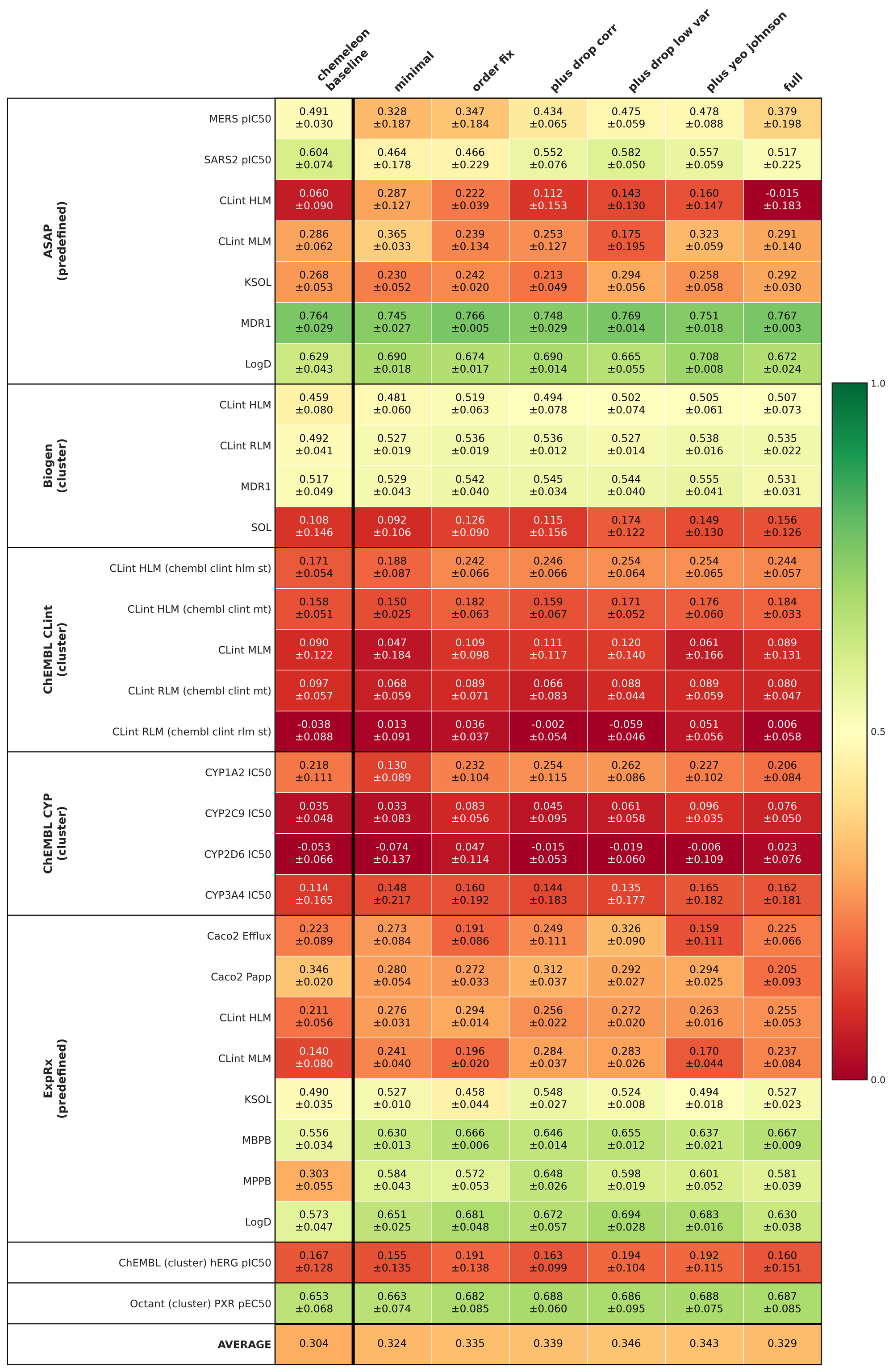
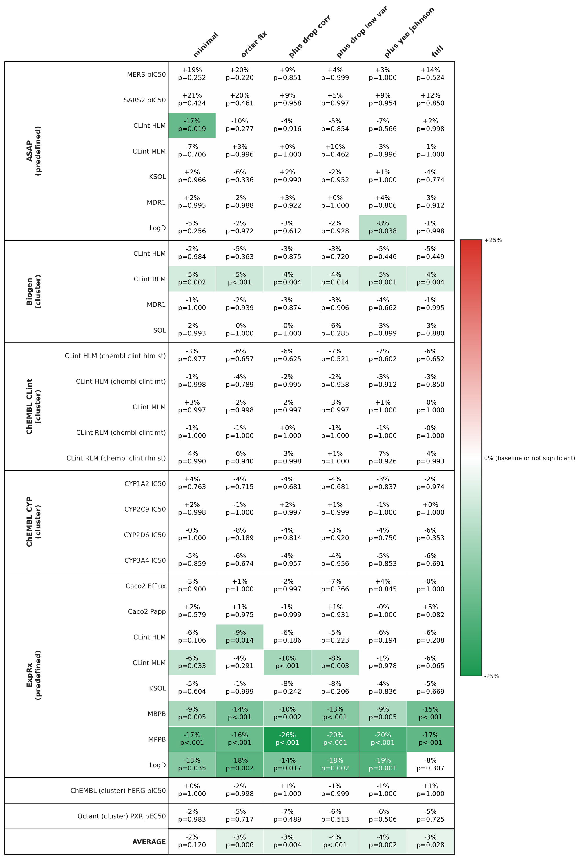
We performed our experiments as a series of ablations of the full prescaling workflow. The ablation set is shown in the table below. We then compared each against the original CheMeleon’s performance, using the weights downloadable from Zenodo. We ran the baseline with twenty random seeds and five random seeds for each condition. These five random seeds randomize the FFN weight initialization, the splits, and featurizer shuffling. To determine the difference in performance, we performed a Dunnett’s test between the baseline and the condition for each cell. The results are shown in the heatmaps below for the R² and the percent change in the mean absolute error (MAE).

Table 2: Ablations

Prescaling ablations showed small, positive results

Although no change to the prescaling scheme improved every endpoint, the sum change was net positive, including for the minimal condition, which consisted only of standard scaling. This may be due to the skewed standard scaling prior to Winsorization that we suspected earlier. With this fix and some pipeline additions, we managed some small performance improvements. However, the magnitude of performance changes in these results was overall rather small, indicating that CheMeleon may already be robust to issues with poorly scaled data. Given this slight improvement across most of our endpoints, we chose to proceed with the “order fix” condition in the following experiments with featurization. For our later datasets, we used the “full” condition–which uses all of our filtering steps–primarily for internal, historical reasons.

Pretraining featurization: What’s the best method?

The original CheMeleon paper pretrained the MPNN on Mordred descriptors computed for their PubChem-curated dataset. These descriptors offer a wide range of different chemical properties for the network to learn. However, there is a vast array of ways to present molecules to a network, ranging from computed chemical descriptors and molecular fingerprints to 3D and quantum methods. In the interest of getting a comprehensive overview, we select 15 different featurization schemes for the original CheMeleon dataset. Most of these methods will be familiar to readers, but there are a few exceptions toward the end of the table.

The first exception is the Novartis surrogate model. This model was created using this data from Novartis, where the data in question was not real assay data, but instead data that had been predicted by a model trained on their highly consistent, internal corpus, hence the term “surrogate.” We wanted to test the use of surrogate data as a kind of “pseudo-descriptor” for pretraining our models, so we ran pretraining directly on the surrogate data. We wanted to ask the question: Is using these more direct ADMET predictions advantageous over computed chemical descriptors? It is important to note, however, that this is the one condition for which we did not use the CheMeleon dataset, and instead used the Novartis data, so the difference in dataset size and chemical space coverage will also bias the results.

The second set of exceptions in our table are the three principal component analysis (PCA) conditions. We wanted to know if training on a set of dimensionality-reduced descriptors would yield the same results as training on the descriptors themselves. We used the same Mordred descriptors as in our baseline model and performed PCA on this set. We made three dimensionality-reduced descriptor sets, with explained variance of 80%, 90%, and 95% by the resulting axes. 

We followed the same experimental setup as in the previous section, using five condition random seeds versus the five baseline seeds, pretraining each condition with a different featurization method. For all 3D methods, single conformers were generated using experimental torsion knowledge distance geometry (ETKDG), followed by minimization with the Merck Molecular Force Field (MMFF94). 

Table 3: Featurization method

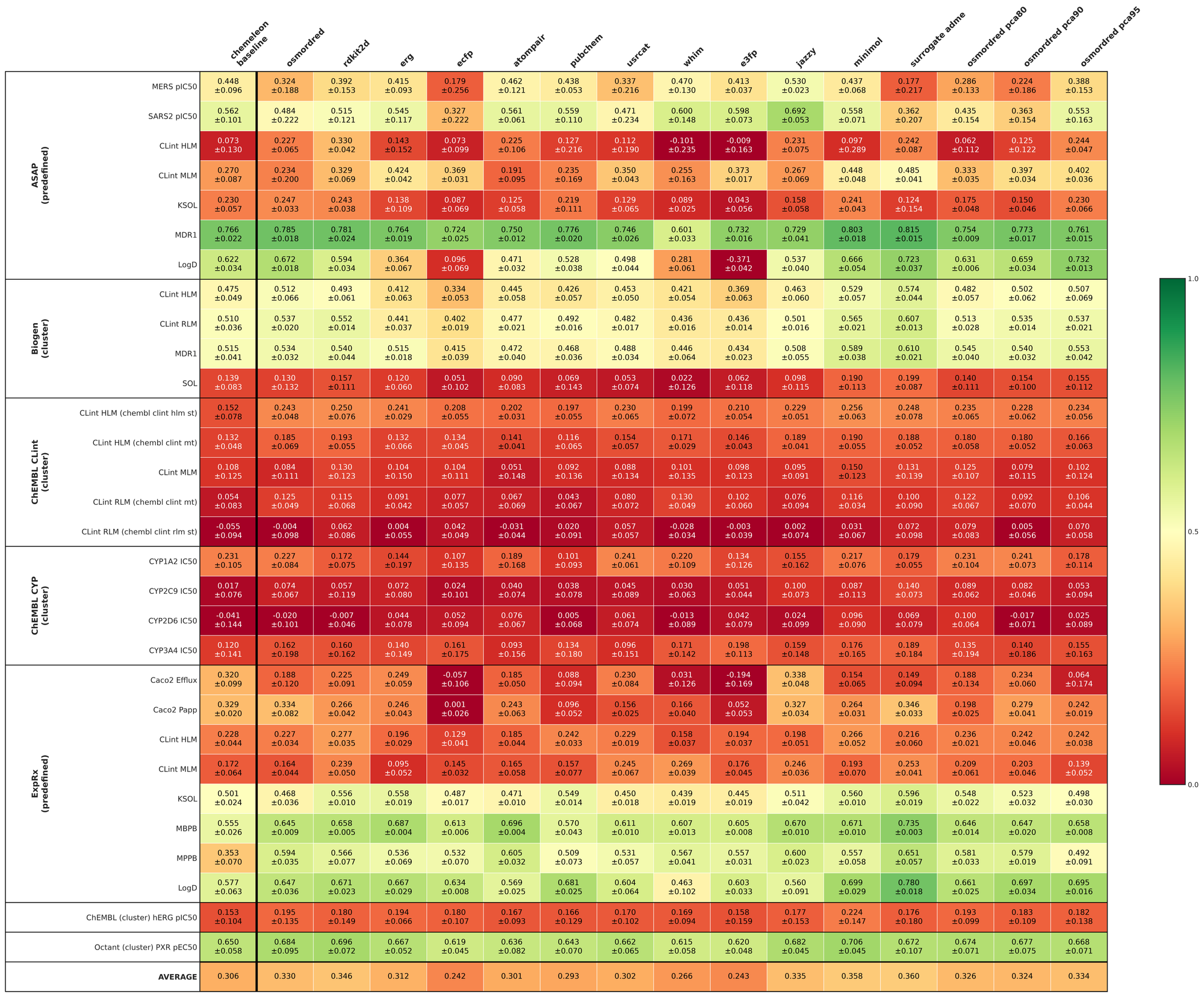
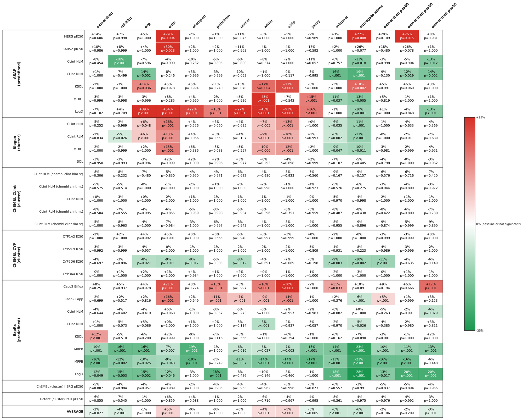
A few featurizers showed small, positive results

No featurization strategy showed statistically significant improvements across all endpoints relative to the original CheMeleon model. However, there were interesting patterns and conditions in which a particular featurization strategy provided additional benefits. 

There were a few strategies that did seem to improve performance across some endpoints. MiniMol was a standout with a net reduction of 6% in the MAE across endpoints. MiniMol itself is a foundational model trained on both quantum and biological tasks, and the “fingerprints” we extracted from it were learned embeddings from the MPNN backbone layer. As the full MiniMol model was shown to have competitive performance in the original CheMeleon paper, the performance boost from pretraining on its embeddings is unsurprising.

The other strategy that provided a similar 6% reduction in MAE was, in fact, not a true featurization strategy at all, but rather the surrogate model, which performed especially well on the ExpansionRx datasets. This is somewhat to be expected, since the “pseudo-descriptors” in this case are in fact ADMET endpoints. Given that this was the only endpoint that used a different pretraining dataset, you could argue that the improvement may simply be due to a difference in chemical space. To test this hypothesis, we ran one additional experiment, comparing how the surrogate data performed against pretraining this same dataset with computed Mordred descriptors. The surrogate data experiments had an R² of 0.369, compared with the osmordred equivalent of 0.305 (p=2e-5), so we conclude that the improvement is, in fact, attributable to the surrogate data itself.

We included fingerprint featurizers primarily as a negative control. Because fingerprints are derivable directly from the graph structure of a molecule, we did not expect to see good performance from these conditions. The RDKit ECFP, and especially E3FP, had very poor performance across many endpoints. Surprisingly, though, some of the other fingerprint conditions, such as atompair and usrcat, had reasonable, though generally worse, performance when compared with the original CheMeleon. In the case of usrcat, this is more understandable, as the 3D conformers are not trivially derivable from the graph structure. However, atompair, like ECPF and many other fingerprint methods, is directly derivable. Even without novel information, CheMeleon still performs well, which speaks to the robustness of the underlying model. But this could also speak to the “hot start” theory we discussed in the introduction, which holds that models aren’t learning any broad foundational chemistry from pretraining but instead merely get a leg up by starting with favorable weights.

It’s also worth noting the results of our PCA conditions. The PCA-reduced Mordred descriptors struggled with some endpoints, particularly given the low explained variance. But at 95% explained variance–a full 93% reduction in descriptor space–there was a net positive effect. As we saw briefly in our prescaling experiments, reducing the amount of extraneous information provided to the model (e.g., by removing low-variance columns during pretraining) appears to have a very small net positive effect in some cases. But again, we see that CheMeleon doesn’t particularly want to budge.

Dataset size and density: which dataset has the optimal chemical space coverage?

As we’ve covered, the original CheMeleon workflow was to select 1M datapoints randomly from PubChem as a pretraining set. We wanted to ask how the size, coverage, and diversity of this dataset alter performance. At first, we believed a larger, more diverse dataset would be the key to improving performance. Since the underlying idea of foundational learning is that the model is learning general chemical understanding, we thought it would behoove us to expose our model to as much chemical variety as possible. After searching the literature for dataset options, we settled on MolPILE, which is a large, diverse set of minimally filtered compounds from researchers at AGH University of Krakow and the Polish Academy of Sciences, compiled from several publicly available datasets. These datasets include PubChem and UniChem, as well as screening catalogs Mcule and ChemSpace, and natural product databases Subernatural3 and COCONUT, with minimal filtering applied. The resulting dataset was then systematically subsampled into datasets containing 1M, 5M, and 10M molecules using a maximum-diversity approach that finds a subset of molecules by maximizing the sum of their pairwise Tanimoto distances. We used each of these sub-datasets as three conditions to determine how pretraining dataset-size affects performance, but we filtered each set to compounds with molecular weights under 500 Da, as we are primarily focused on small molecules.

We also wanted to ask what might happen if, instead of providing the network with a more diverse dataset, we provided it with an extremely dense, targeted one. Our thoughts about providing diversity to the model were, of course, only hypotheses. It could be that learning general knowledge in a region of interest is more a matter of filling in gaps in that space, rather than throwing a large variety of chemical matter at a model and potentially confusing it. Generative methods have been of interest for exactly this kind of application. These methods allow us to algorithmically generate large datasets of molecules from compounds we are already interested in. Could these be used to train foundational models? We decided to test this theory. 

Generative models can be finicky to work with, as many will generate molecules that are chemically impossible. We chose ANNalog, a method we found to effectively filter out problematic molecules, such as those with nonsense ring structures. We generated this data for our ExpansionRx challenge training set to see whether we could improve performance on that set, and to observe how performance changes across other sets. We generated 200 SMILES strings for each member of the ~5000 compound training set. Then we filtered out duplicates, resulting in a relatively small 40k-SMILES pretraining set.

We prescaled our descriptors for both the MolPILE conditions and the generated dataset using the “full” setup described in the prescaling section. Then, we ran our experiments with the same endpoints as from the previous experiment sets above.

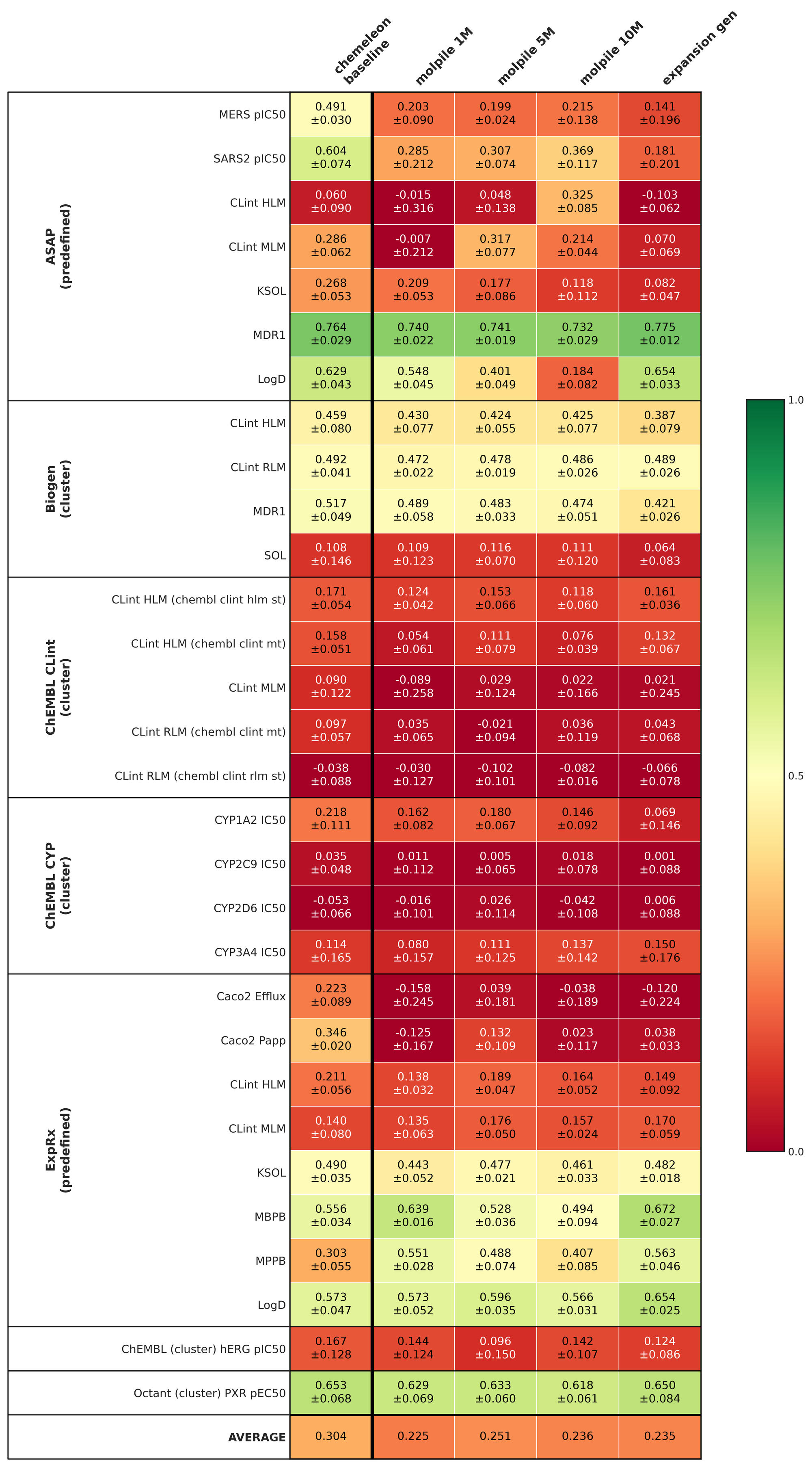
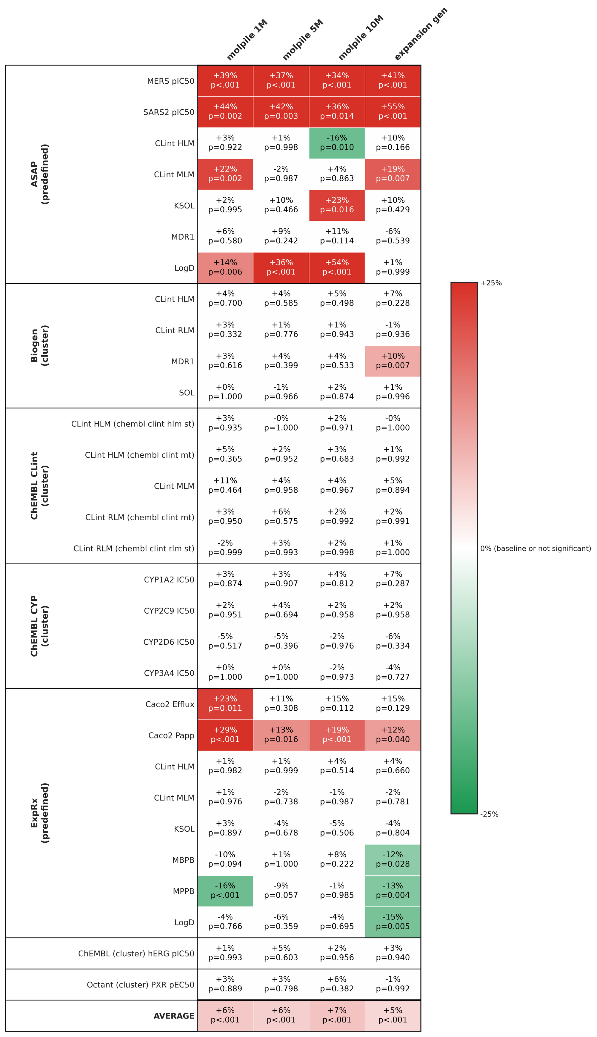
All of our datasets decreased performance

Unfortunately, the diversity of MolPILE failed to deliver many significant results. In most cases where there was change, MolPILE pretraining was a significant disadvantage relative to the original CheMeleon. The sparsity of MolPILE, rather than providing the model with broad chemical intuition, probably instead made it difficult for the model to intuit properties. We clustered the original CheMeleon PubChem data, combined with the MolPILE data, to investigate this. There was overlap in chemical composition between sets, but almost all MolPILE-only clusters were singletons, compared to CheMeleon-only clusters, which averaged 90 molecules. These results support our hypothesis that the extreme diversity was a hindrance, rather than a help.

The Expansion-generated set performed reasonably well on the Expansion endpoints, which was surprising, given the prevailing theory that foundational learning comes from a network learning more “general” information. Additionally, it was surprising that the Expansion-generated set didn’t seem to decrease performance on other endpoints particularly strongly, despite having a pretraining set confined to such a narrow range of chemical space. In fact, by a small margin, the Expansion-generated set outperformed the 10M MolPILE set overall! Though the precise reasons for this are unknown, these results suggest that more diversity is not always better and that providing a network with a pretraining set that reasonably covers the space you’re interested in is more important. 

The overall result from this section, as with others, is that even large perturbations to the underlying dataset don’t seem to impact performance terribly much. It is difficult to draw sweeping conclusions, as there is a huge amount of complexity baked into dataset choice. But we suspect that altering the dataset, even increasing its size severalfold, is unlikely to significantly improve performance. In the next section, we’ll look at work from the Green Group at MIT on architecture changes.

Architecture Experiments

In parallel with OpenADMET’s work to improve CheMeleon's performance by experimenting with the data, the Green Group at MIT conducted experiments on the architecture itself. Guided by OpenADMET, we moved toward the same larger datasets and descriptor sets described above, eventually settling on MolPILE and Osmordred. We theorized that the standard D-MPNN architecture would not be sufficiently expressive to learn from the additional data, though, and tried multiple strategies to address it.

Literature-derived Message Passing Schemes 

Many other GNN architectures have been published in the scientific literature, each with its own message-passing scheme. One in particular stood out in the original CheMeleon study: MiniMol. This foundation model offered competitive performance with both CheMeleon and the strongest random forest baseline, suggesting that its representation learning strategy was a promising avenue for investigation.

More specifically, MiniMol states in their paper that they use GINE message passing, which can be thought of as a variant of Chemprop’s BondMessagePassing with more parameters for each update. Using Gemini, we translated their original implementation into a Chemprop-compatible class, then ‘plugged it in’ to the Chemprop v2 API.

The MiniMol study also evaluated the MPNN++ message-passing algorithm. This approach also incorporates global features within each message-passing iteration, granting it a high performance ceiling. The MiniMol authors observed that simply increasing the hidden size of GINE message passing was more effective than switching to the more expressive MPNN++ message passing algorithm (within a fixed parameter budget). Given that we have as much pretraining data as we need and there is no size constraint, we included this approach as well.

Novel Message Passing Schemes 

Beyond simply pulling existing schemes from the literature, we also implemented new algorithms to address specific limitations of the D-MPNN framework: over-regularization and a lack of expressivity. Both of these avenues of investigation are inspired by the foundational Neural Message Passing for Quantum Chemistry paper, which is still a worthwhile read more than ten years later.

First: regularization. During message passing, the same matrix is reused for every iteration (i.e., depth in Chemprop). This regularization strategy forces the model to reflect the physical argument that the hidden-state update function should remain consistent regardless of the perceptual field’s size. Empirically, the authors state that it simply performs better. Again, given that we now have so much data, can we relax this and exploit the ability to learn a depth-specific update function?

Second: expressivity. During every message-passing iteration, each atom simply sums the incoming messages from its local neighborhood. In reality–and especially for some properties–you want the message-passing scheme to focus on certain atom types or groups of atoms (e.g., functional groups) rather than a naive sum. This is analogous to the GAT architecture (described here), but Chemprop-compatible.

Autoresearch for Hyperparameter Optimization 

This combination of many different message-passing schemes led to a new challenge during our experimentation: the model's design space was now massive. We had to choose one of five message-passing schemes, each with unique hyperparameters, along with the typical Chemprop hyperparameters such as learning rate and FFN size. This was far too challenging for manual investigation, and brute force enumeration was impractical.

To address this, we turned to autoresearch, Andrej Karpathy’s framework in which a Large Language Model (e.g., Gemini) iteratively attempts to improve model performance by directly modifying the pretraining code. The key advantage this has over typical hyperparameter optimization is flexibility–the LLM can deal with variable hyperparameter sizes and make one-shot suggestions using its prior knowledge, all without requiring the additional, somewhat complex programming needed to use traditional hyperparameter optimization in this application. 

Note that “model performance” in this case is different from the original autoresearch formulation, which sought only to improve pre-training performance. Instead, for this study, Gemini was instructed to conduct pretraining and then run the pretrained model through an evaluation script. This script uses Polaris to fine-tune the model on a subset of the original CheMeleon benchmarks, returning the average of test set polaris/pkis2-ret-wt-cls-v2 ROC-AUC, polaris/adme-fang-solu-1 R², tdcommons/clearance-hepatocyte-az Spearman Rho, and tdcommons/bbb-martins ROC-AUC.

This subset was selected because online fine-tuning on the entire benchmark dataset was computationally impractical and because the standard approach of optimizing on the pretraining performance did not work (you’ll see why in a moment).

Autoresearch Results

First and foremost, the autoresearch was successful in improving the model on the pretraining objective. Figure 8 shows the LLM's improvement in the pretraining objective over ~50 experimental iterations. This exact run did not consider the entire design space mentioned above, but is representative of the results across our various experiments.

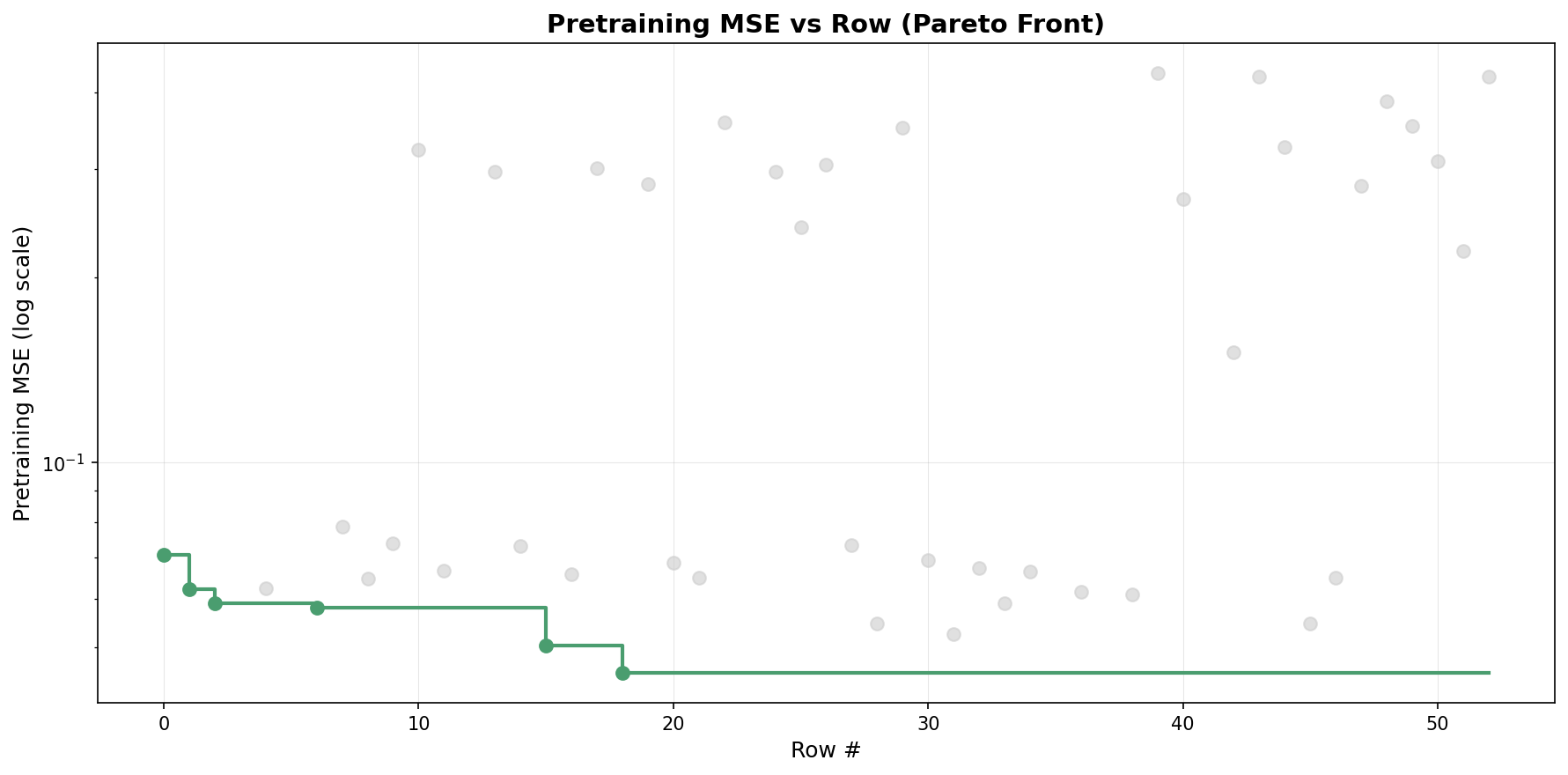
The baseline initial run (configured by us) achieved a relatively good pre–training MSE of 0.07. As the LLM worked, it reached its best performance at 19 iterations, with a score of 0.045 (a 36% improvement!). As the experiment progressed, the model also generated some much worse results as well, which we think is good–after it made the ‘easy’ modifications to achieve better performance, it tried more radical changes.

…and that’s where the good news ends. When we actually look at the fine-tuning performance–small, insignificant improvements.

Let’s now look at our fine-tuning performance metric vs. iteration in Figure 9. The model improves from 0.61 to 0.66, a less than 10% gain over the training lifetime.

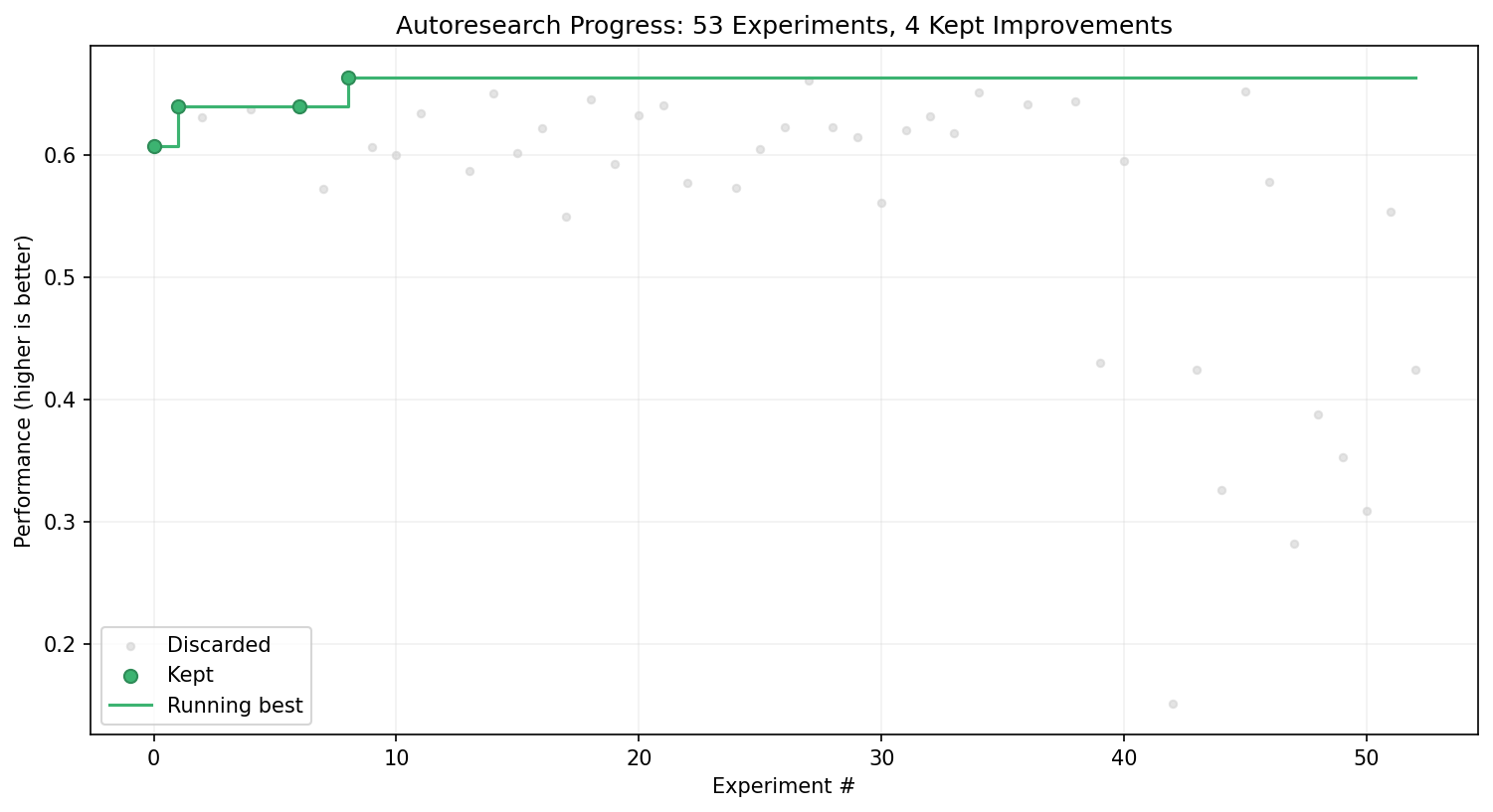
This reaffirms the observations made above regarding robustness. The CheMeleon pretraining approach is apparently rather insensitive to our decisions made during pretraining. This carries over to the full benchmark set as well. When we applied the final model from this autoresearch run to the entire benchmark set, the results were not statistically significantly better than those of the original CheMeleon model.

Worse still for our efforts in improving CheMeleon, Figure 10 demonstrates the core challenge in this optimization that we alluded to earlier: pre-training performance is a poor proxy for fine-tuning performance.

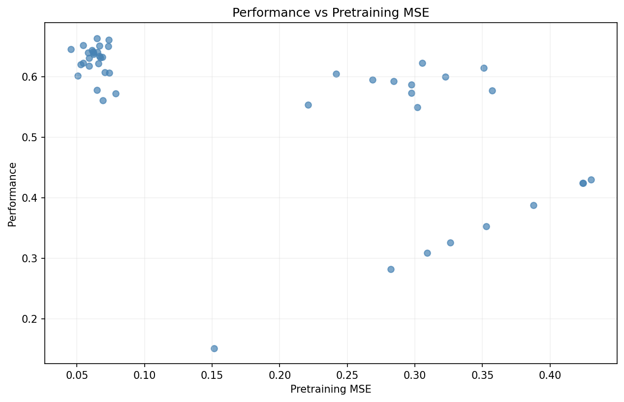
While it is true that all the best-performing models have a pretraining MSE below 0.10, there are still models with pretraining MSE exceeding 0.30 that achieve comparable performance. This spells doom for any optimization process–classical or LLM-driven–because of a poor signal.

We will stop here for now rather than repeat more plots showing equal-or-worse performance on our benchmarks. Suffice it to say that many iterations of message-passing architecture development, autoresearch, and dataset exploration did not yield a ‘CheMeleon2’.

Conclusions

Though our results failed to return any statistically significant, across-the-board improvements, there were a few improvements on individual tasks. These improvements warrant further investigation, but overall we conclude that the CheMeleon pre-training strategy is robust to hyperparameter choices and pre-training methodologies. In some ways, this is a good thing–there’s no need to be worried about finely tweaking parameters to boost performance when seeking improvements on individual tasks. On the other hand, this also means that a generally improved ‘CheMeleon2’ is difficult to achieve without departing from the D-MPNN framework. 

All of the changes described above fall broadly into the category of ‘changes which could conceivably be introduced to Chemprop and made available without requiring a new major version.’ The literature suggests (see this work) that relaxing this constraint and moving toward tabular foundation models built on top of the CheMeleon fingerprint could further improve performance. 

While this venture did not result in the release of a new and improved CheMeleon 2.0, we hope that it is a valuable exercise to share with the community at large. The journey towards model improvement is a long and winding road, full of dead ends. Too often, work like this goes undocumented. We hope that by reporting negative results, we can encourage others in the community to share similar work, so we can all learn from each other’s mistakes and reduce duplication of effort. We will also share our checkpoints from the featurizer experiments here, as well as the code for all dataset experiments and architecture experiments. We encourage you to try some of our checkpoints out for yourselves and report back. If you’d like to join us on the island of misfit models, we’d encourage you to reach out! Do you have a set of experiments gathering dust in a folder somewhere? We’d love to hear about them! Please reach out to Devany West or Jackson Burns with any questions about this work.

Acknowledgments

We would like to thank our funders for their support of OpenADMET, in particular ARPAH, Radial (part of the Astera Institute), Schrödinger Inc, and the Gates Foundation. We would also like to thank our partners Enamine, HuggingFace, OpenEye, CDD Vault, Discovery Life Sciences and the beamline staff at NSLS-II for their support.

This work is supported by the Advanced Research Projects Agency for Health (ARPA-H) under AVOID-OME, and Award Number 1AY1AX000035. The contents are those of the authors. They may not reflect the policies of the Department of Health and Human Services or the U.S. government. The content is solely the responsibility of the authors and does not necessarily represent the official views of the Advanced Research Projects Agency for Health.

JWB gratefully acknowledges financial support from the U.S. Department of Energy, Office of Science, Office of Advanced Scientific Computing Research, Department of Energy Computational Science Graduate Fellowship under Award Number DE-SC0023112. This research used resources of the Oak Ridge Leadership Computing Facility at the Oak Ridge National Laboratory, which is supported by the Office of Science of the U.S. Department of Energy under contract no. DE-AC05-00OR22725.