Tune In: What Fine-tuning OpenFold3 Taught Us

Author: Kate Huddleston

DOI:

Foundational cofolding models, like OpenFold3 and Boltz-2, are trained on massive datasets at high computational cost. In the process, they encode the common patterns found in protein and ligand structure space, achieving impressively accurate structure predictions for some targets. For targets where cofolding underperforms, fine-tuning on experimentally determined protein-ligand structures of those targets may help close the performance gap. 

How does fine-tuning work? 

When a model has consistently high failure rates, fine-tuning is the standard way to improve performance. Fine-tuning adapts a broadly trained foundation model by updating its parameters with curated structural subsets, such as specific target families, protein-protein interfaces, or protein-ligand complexes. The aim is to improve the model’s performance on your use case, without losing the broader structural priors learned during initial training. This method is appealing: if you have even a small number of high-quality structures for a difficult target, fine-tuning offers a way to specialize a general model without incurring the prohibitively high computational cost of training one from scratch. While it takes 256 GPUs and about 3 weeks of compute to train OpenFold3 from scratch, we fine-tuned our models with a single GPU in a matter of hours to about a day, depending on training set size. 

At OpenADMET, we believe that predicting the structures of small molecules bound to Avoid-ome targets is critical for understanding structure-function relationships and mitigating ADMET liabilities. Off-the-shelf cofolding models on these targets had limited success. In our early attempts, only about a third of the structures in our CYP3A4 and PXR benchmarks were predicted with a ligand pose within 2.0 Å of the experimental pose. 

A large part of our project is devoted to generating high-quality assay and structure datasets, as public data for ADMET targets is scarce and inconsistent. Currently there are only 74 ligand-bearing PXR structures in the PDB, all from different sources and of different resolutions. Over the past year, our collaborators at UCSF have built the largest public PXR structural dataset to date, consisting of 184 crystal structures. We released this data as part of our PXR blind challenge, which ran from March 17 to July 1 of this year. Naturally, we asked ourselves whether we could leverage this dataset to improve cofolding predictions for PXR. To achieve this, we set out to fine-tune OpenFold3 for PXR, with close help from the OpenFold team.  

Fine-tuning a model to be the all-knowing PXR structure expert, or even just a mediocre predictor, turned out to be no easy feat. Some of our attempts helped a little, but most resulted in more questions than answers. This led us to look for what had actually worked in published fine-tuning efforts on other targets, to understand not just whether performance moved, but also why.

The science of fine-tuning a cofolding model is still in its infancy. The following is a comprehensive overview of what we have learned through this process, as an attempt to turn this new art into a science. 

Successful fine-tuning attempts

In the past year, two important blog posts have been published evaluating the potential of fine-tuning OpenFold3 on structural data the model has never seen: 

• “Fine-tuning OpenFold3 on a small set of structures: The PDE10A case study” published by Apheris 
• “OpenBind’s first release: A structure-affinity dataset for structure based AI” published by OpenBind

Apheris, a company focused on federated fine-tuning for drug discovery, evaluated fine-tuning with a subset of 27 PDE10A (a phosphodiesterase enzyme) structures from the Protein Data Bank (PDB) (10 in train and 17 in test), all of which were held out from the baseline OF3 training. The team at OpenBind, an initiative which builds open-access drug-protein interaction datasets, looked at the Enterovirus A71 (EV-A71) 2A protease, fine-tuning on a subset of 79 internal fragment structures and testing on a set of 63 follow-on compounds. 

Both reported improved ligand pose prediction compared to the baseline model on their test structures. So we expanded our scope from “Does fine-tuning work?” to “What makes it work?” and “Why isn’t it working for us?” 

How much does similarity matter? Defining “same-pose coverage” pairs.  

To better understand the successes of Apheris and OpenBind, we began by exploring their training and test sets, focusing primarily on chemical self-similarity. In their recent paper  “Have protein-ligand cofolding methods moved beyond memorisation?”, Škrinjar et al. showed that several cofolding methods succeed only when the ligand and pocket structure have high similarity to the training set. Maybe fine-tuning only helps when the ligands in the complexes resemble those in the training set, and our data is just too diverse? 

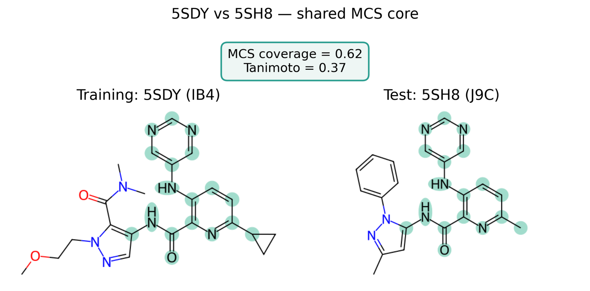
We first measured how similar the ligands in each training set were to those in the corresponding test set. Ligand similarity is typically measured using whole-molecule metrics such as the Tanimoto coefficient. We expected the test sets to look meaningfully similar to the training sets under this metric, as these are cases where fine-tuning worked. However, we noticed a more helpful trend at the substructure level. To capture substructure similarity, we used the Maximum Common Substructure (MCS), which measures the largest connected set of atoms shared between two ligands. 

To clarify this choice, let’s look at an example. Figure 1 shows two ligands from the PDE10A case study, one from training and the other from test. This train-test pair shares a structural core of 18 heavy atoms, which is 62% of the smaller ligand’s atoms (its MCS coverage). Yet their whole-molecule Tanimoto similarity is only 0.37, indicating a weak, although significant, similarity. 

Say we were asked to predict whether this training structure would help the model succeed on this test structure, and were only given the Tanimoto value. Our guess would have been “probably not.” But as you will see, that would have been the wrong answer. 

The pattern we found, and will focus on for the rest of the post, is what we are dubbing "same-pose coverage." A train-test structure pair has same-pose coverage when it meets the following criteria: 

1. The pair shares a heavy-atom core.
2. The shared core adopts the same pose within the binding site.

We performed a sweep across a range of same-pose coverage criteria, from strict to loose, tracking both how many pairs qualified under each and how many distinct training structures those pairs traced back to. At the strict end, a pair needs to share a core of at least 12 heavy atoms within 1.5 Å; at the loose end, a core at least the size of a benzene (6 heavy atoms) within 2.0 Å qualifies. Figure 2 shows the results of this sweep for both of the targets from the fine-tuning reports, PDE10A and EV-A71 2A. The x-axis labels the coverage criteria. The y-axis shows the percentage of the test set—17 ligands for PDE10A and 63 for EV-A71 2A—that has at least one training structure meeting that criterion. Each bar is stacked and colored by the training structure that provides the match, so a bar’s total height represents overall coverage, and each colored segment shows one structure’s individual share. The number below each percentage is the count of distinct contributing training structures. 

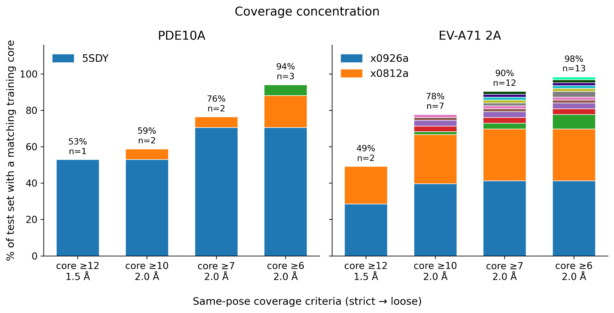
PDE10A’s test set coverage traces back to a single training structure, 5SDY, at every threshold we checked. EV-A71 2A’s coverage is spread across two co-dominant fragments, x0926a and x0812a. The EV-A71 2A protease data coverage looks more distributed than PDE10A, spanning from 2 to 13 contributing fragments across the sweep against PDE10A’s 1 to 3. But relative to each pool’s actual size, EV-A71 2A reaches comparable or higher coverage while drawing from just 16.7% of its own training set, versus 30% for PDE10A. In both cases, a handful of training structures cover roughly half or more of the test set at every threshold we checked. 

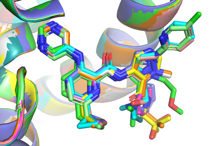
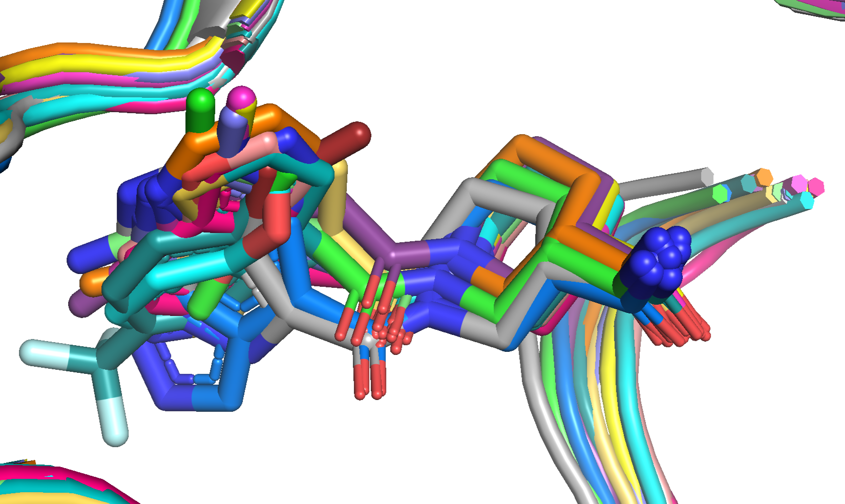
To see what coverage looks like structurally, Figure 3 overlays same-pose coverage test set structures with 5SDY (Figure 3.a) and x0926a (Figure 3.b), both shown in green. In both cases, the shared cores consistently occupy the same location and pose across every member.

a)

b)

To test whether the presence of these keystones, or dominant training structures, correlates with model success on the test sets, we ran an ablation experiment. For each case study, we fine-tuned three different models trained on: 

• the full training set
• the full set with the keystone(s) removed
• the keystone(s) alone 

We evaluated each model against the same established test set from its case study, using ligand BiSyRMSD (Figure 4). For PDE10A (Figure 4.a), every fine-tuned model outperforms the baseline on average, including the model trained without the keystone structure. However, the two models whose training sets included the keystone have visibly tighter distributions than either the baseline model or the model trained without the keystone, whose overall distributions are broad and comparable. For EV-A71 2A (Figure 4.b), the same overall trend holds: models trained with the keystones present have tighter RMSD distributions than those without. 

a)

b)

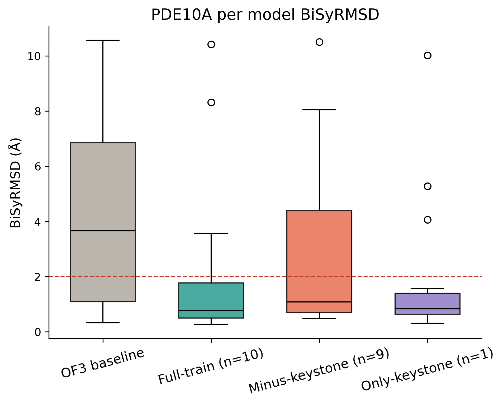
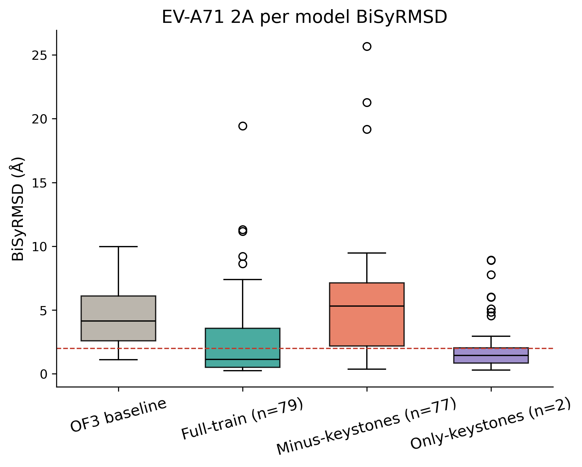
In both cases, the keystone-only model performs best. This effect is especially pronounced in the EV-A71 2A case, where adding the rest of the training set actively hurts performance rather than simply contributing less. Across both ablation experiments, the fine-tuned model’s real signal comes from training structures that are highly similar in structure and geometry to the test set. 

These two cases reflect the same phenomenon at different scales. Both show that the raw number of training structures does not matter. Cofolding models can benefit from exposure to multiple structures in their fine-tuning dataset, but what matters is how much of the training and test sets share same-pose coverage. 

Does a same-pose coverage split hold for PXR? 

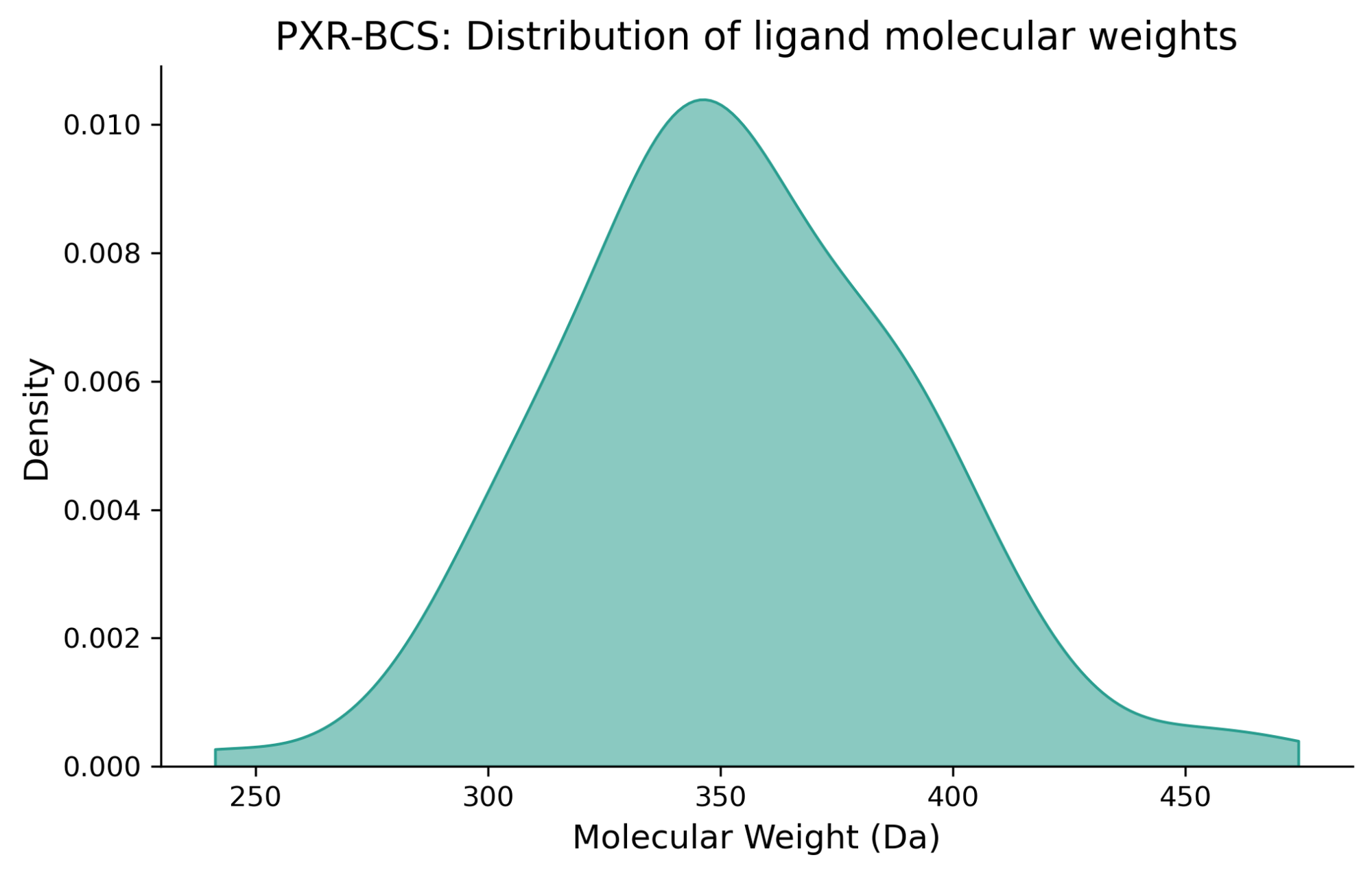
The PXR dataset, generated by UCSF as a part of the OpenADMET consortium, consists of high-quality X-ray crystal structures spanning 184 molecules ranging from fragment-sized compounds to drug-like ligands. For this analysis, we used a subset of the full-ligand structures from our PXR Blind Challenge set. For the remainder of this post, we will refer to this set as PXR-BCS. Figure 5 confirms that this subset is drug-like, as opposed to fragment-like, throughout, with a molecular weight range of 241-474 Da. 

In both case studies discussed above, we found that keystones are central to the success of fine-tuning efforts. In our first attempts at fine-tuning on PXR, we did not see the promising results we were expecting, despite having a large amount of high quality data. To investigate this, we asked whether common substructures exist in the PXR dataset and whether they share a common pose. In other words, were keystone structures present within the PXR dataset?  

We performed a same-pose coverage split on PXR-BCS using the same strict coverage criteria as shown in Figure 2 - a shared core of at least 12 heavy atoms within 1.5 Å. In contrast to PDE10A and EV-A71 2A, there were no obvious training keystones for the full 89-structure set, as any groups with same-pose coverage were only made up of about 2 to 5 compounds. With limited similarity between structures, we could not repeat our keystone ablation experiment for the PXR series.

So instead, we compared the performance of a model fine-tuned on a naive random split with that of a model fine-tuned on a curated same-pose coverage split. From the same-pose coverage available in the data, we hand-selected 8 keystone structures for our training set based on nearest-neighbor same-pose similarity. To establish a validation set, we identified 19 ligands that met our coverage criteria against at least one of the training structures. All validation structures were distinct from their covering keystone, ensuring no data leakage. This design, while unrealistic, was made to evaluate the best-case scenario. 

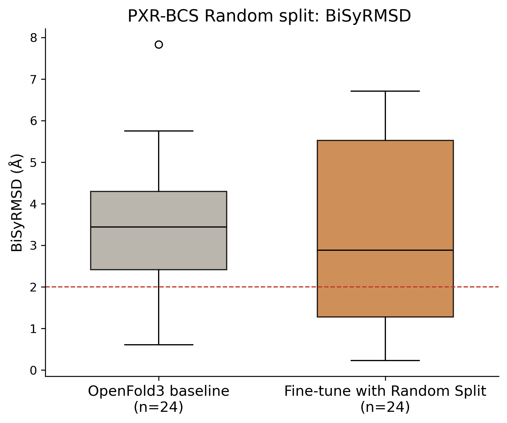
Based on the RMSD distributions in Figure 6.a, we observe that fine-tuning on a random subset of PXR structures did not yield any performance improvement on a random test set.  While the median RMSD dropped slightly, the distribution became wider, and RMSD increased for several structures. 

We evaluated the model fine-tuned on our same-pose coverage split across three different test subsets: the 19 covered validation structures, the other 70 held-out structures from our PXR-BCS subset, and the full 89-structure set exempt from training (Figure 6.b). We found the performance differences between subsets to be sharp. Fine-tuning on our same-pose coverage split clearly improves ligand pose prediction on our curated validation set. That gain steadily shrinks as same-pose coverage disappears, with the held-out set having the highest error. 

a)

b)

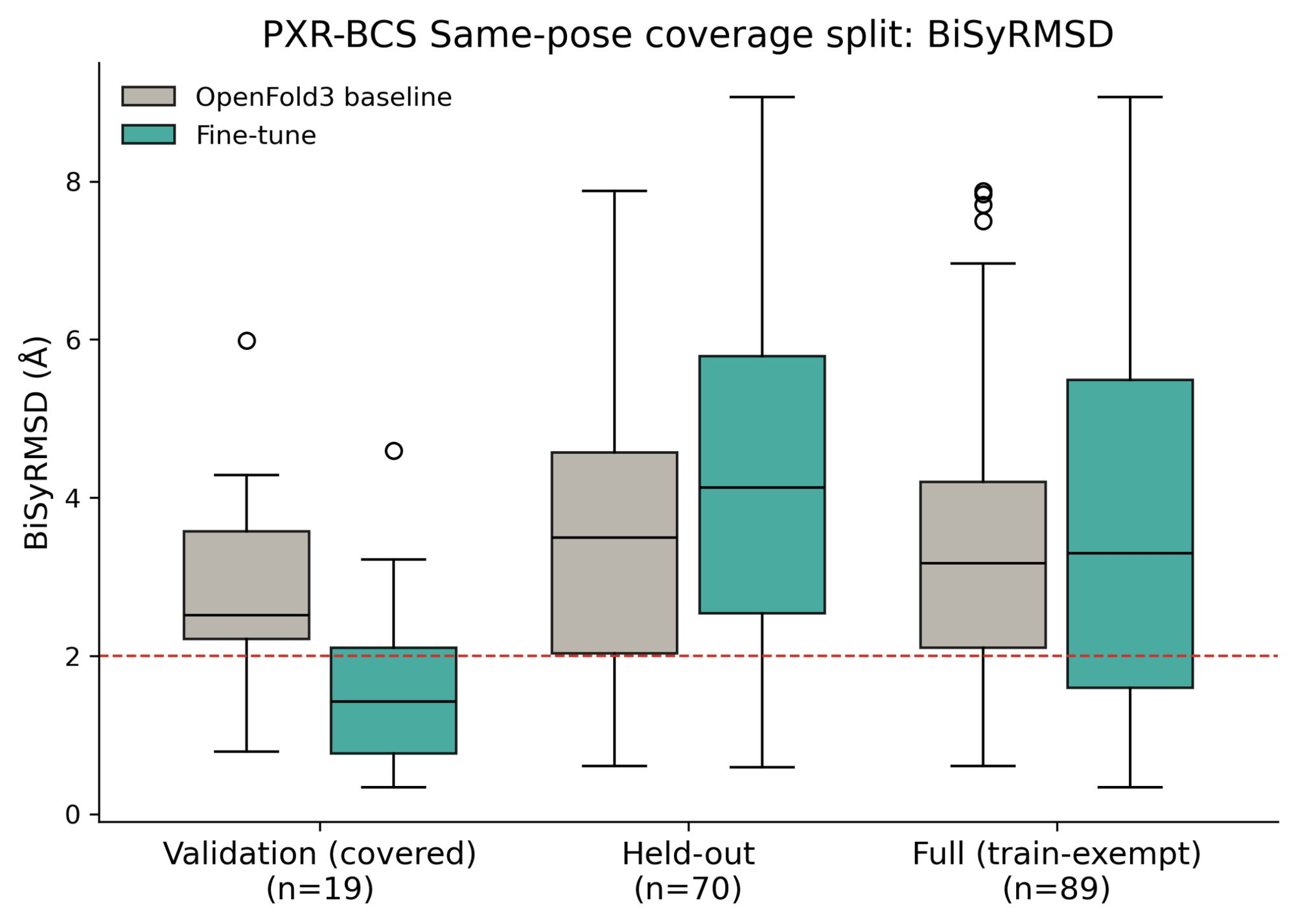
 This matches the same trend we confirmed in PDE10A and EV-A71 2A: the model’s real signal comes from same-pose coverage. But we can’t always depend on building a split like this, especially for promiscuous ADMET targets, where same-pose coverage may not be straightforward to find.  

Same scaffold, different pose

PXR has a large, promiscuous binding pocket, and we have observed considerable variability in how ligands bind within it. Figure 7 examines pose consistency within the scaffold series for each training keystone structure used in our PXR-BCS same-pose coverage split, as well as those from the two published case studies by Apheris and OpenBind. For each of our training keystones, we grouped all dataset members that share a substructure of at least 12 heavy atoms with it, then measured the RMSD of that shared core. This shows how often a shared scaffold actually holds its pose rather than assuming it by construction. 

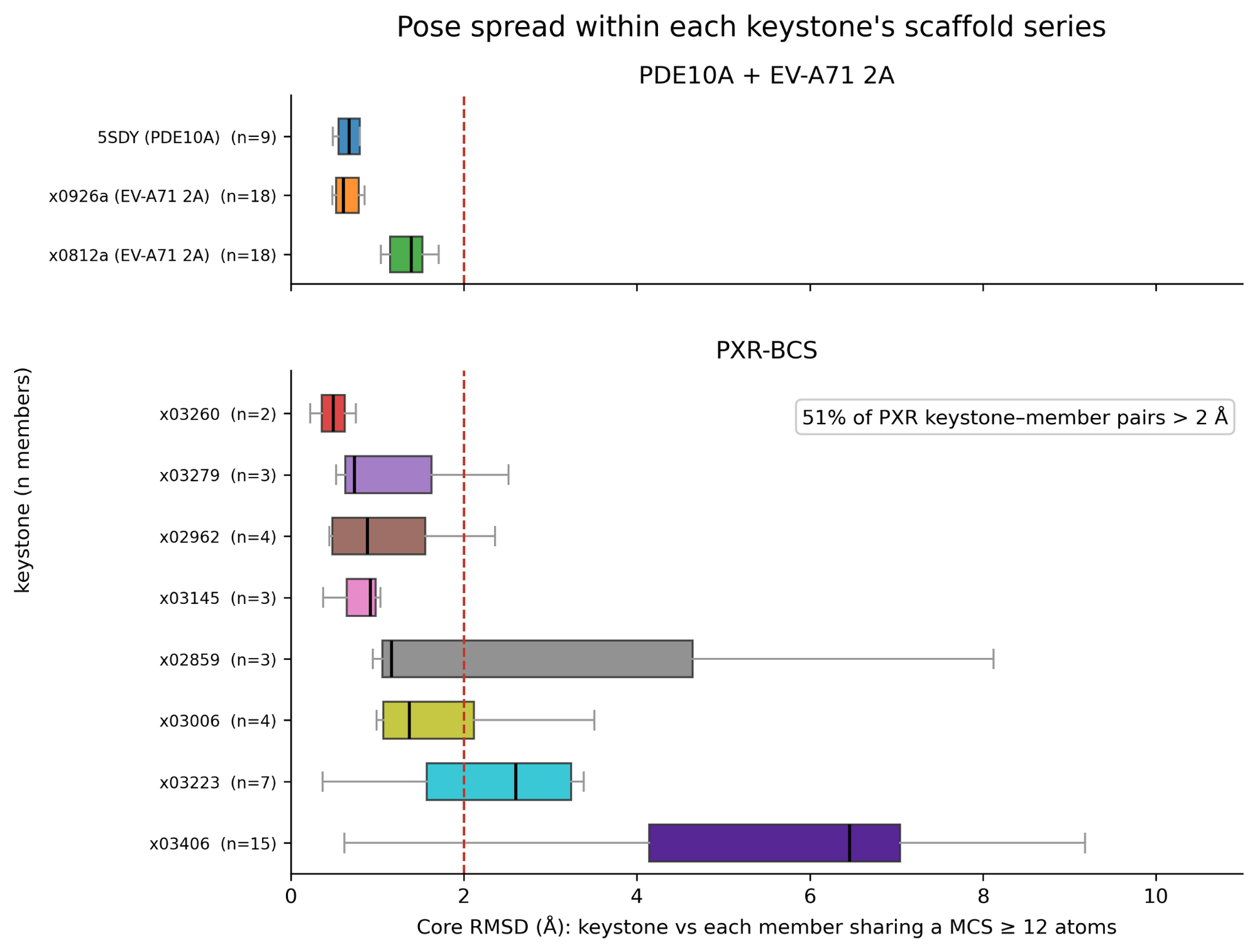
The contrast is stark. PDE10A’s and EV-A71 2A’s keystones maintain a consistent pose across all members of their scaffold series, with RMSD below the 2.0 Å threshold. Our PXR keystones do not. In 51% of all keystone-member pairs, the pose difference exceeds this threshold. It is basically a coin toss whether or not a PXR structure with a shared scaffold will also share a pose. 

This is the clearest explanation we’ve found for why fine-tuning on our PXR data without a deliberately curated split failed. It makes sense in the context of what these models are learning: they are not learning chemistry, but where atoms and residues should sit in space relative to each other. If your training data shows the same substructure binding in different locations, there is no consistent spatial lesson for the model to learn. It is a bit like trying to train a dog to sleep only on his bed while still letting him sleep on the couch and the recliner. The inconsistency itself is the problem, not the volume of data. 

Closing thoughts

Fine-tuning a cofolding model works when the training set gives it a structure to imitate. From our findings, it appears this imitation is rooted in two criteria: the training structure must a) share a common core structure and b) occupy the same pose in the binding site. Unfortunately, while our PXR structures satisfy the first constraint, most fail the second. To achieve truly effective fine-tuning on our promiscuous anti-targets, we may need to develop methods that are less sensitive to these constraints. 

There is still a lot we don’t understand about ADMET targets and about what cofolding models learn from fine-tuning. That said, the observed trend suggests that these models learn spatial signals rather than chemistry, a conclusion consistent with recent work on cofolding mechanisms. It also supports a commonly made point in the field: we need physics-informed models, not just more data.

Acknowledgements 

We would like to thank our funders for their support of OpenADMET, in particular ARPA-H, Radial (part of the Astera Institute (https://ror.org/00ydx1s47)), Schrödinger Inc., the Gates Foundation and the OpenAI Foundation. We would also like to thank our partners Enamine, HuggingFace, OpenEye, CDD Vault, Discovery Life Sciences, and the beamline staff at NSLS-II for their support.

This work is supported by the Advanced Research Projects Agency for Health (ARPA-H) under AVOID-OME, and Award Number 1AY1AX000035. The contents are those of the authors. They may not reflect the policies of the Department of Health and Human Services or the U.S. government. The content is solely the responsibility of the authors and does not necessarily represent the official views of the Advanced Research Projects Agency for Health.